universal algebra – Dan Marsden

Lawvere Theories

In many previous posts, we have discussed connections between monads and universal algebra. So far, we have seen that given a presentation $(\Sigma,E)$ of an algebraic theory in terms of set of operations $\Sigma$ , and equations $E$ , there is a corresponding monad $\mathbb{T}$ such that:

The Eilenberg-Moore algebras of the monad are the algebras described by the chosen presentation.
The Kleisli category is the full subcategory of free algebras.

Many other aspects of monad theory can then be stood from this algebraic perspective.

Every monad arising from a presentation in terms of operations and equations is finitary. This is a technical condition saying that certain colimits are preserved by the monad endofunctor, but we will not dwell on the precise details. Intuitively, the idea is that the functor is completely defined by its action on finite objects. The key point is that there is a correspondence between algebraic presentations and finitary monads, for which the categories of algebras coincide. It is essential that the categories of models agree for this relationship to be algebraically meaningful. Note this is not a bijection, as a given finitary monad will have infinitely many potential presentations in terms of operations and equations.

In this post, we will see a third perspective on describing algebraic structures, Lawvere theories. These sit somewhere between conventional universal algebra and monads in their level of abstraction. As with any mathematical phenomenon, each new perspective deepens our understanding, and emphasises new features and intuitions.

The Idea of Lawvere Theories

To be concrete, lets consider what we need to do to describe a monoid. The general situation for different algebraic structures will follow in the same way.

Typically, we first pick out an underlying set $M$ , and two functions:

A zero argument function, or constant, for the unit element. We can identity this as a function $1 \xrightarrow{z} M$ .
A two argument function, or binary operation, for the monoid multiplication. We can identify this with a function $M \times M \xrightarrow{m} M$ .

Of course, once we have these functions, we can build further ones by combining them together. For example

$M \times 1 \xrightarrow{m \circ (z \times \mathsf{id}_M)} M$

Which informally we can think of as corresponding to a term $m(z,x)$ . Of course, by one of the monoid unit axioms, we require that this composite is equal to

$M \times 1 \xrightarrow{\pi_1} M$

which we can think of as corresponding to a variable $x$ . So in this way of describing a monoid, we:

Pick out some basic operations, which are maps of the form $X^n \rightarrow X$ .
Build lots of other operations by composing the basic operations together, using category composition, and the properties of products.
Require that certain of the operations are equal.

We note some issues with this naive plan. Firstly, where did the basic operations come from, and why do we distinguish them from the other operations? This bias towards certain operations seems categorically unnatural, and raises the ugly question of whether any further mathematical results we derive might be dependent on our choice of presentation. Secondly, a small but annoying detail. It was a pain that $M \times 1$ was only isomorphic, and not equal to $M$ when we built our composite terms. If we build up more complicated composites involving higher Cartesian powers, we will spend a lot of time bookkeeping how to bracket expressions like:

$M \times ((M \times M) \times M)$

for no practical benefit. So putting all this together, it would be convenient if we could describe the theory of monoids as a category with:

Objects the natural numbers, corresponding to the number of arguments of our operations.
(Strict) finite products are given by adding the required arities together $m \times n = m + n$ .
Intuitively, we consider an operation of arity $m$ to be a morphism of type $m \rightarrow 1$ . For example, a binary operation is a morphism $2 \rightarrow 1$ and a constant is a morphism $0 \rightarrow 1$ . Notice that, unlike the common convention, in this case $0$ is the terminal object.
A family of $n$ such operations is a morphism of type $m \rightarrow n$ . This is automatic from universal property of the assumed strict finite products.
A diagram commutes in our category if and only if the corresponding operations should be equal in the theory of monoids.

In fact, it is technical important to add a little bit more structure. If we consider the category of sets, and take the full subcategory with objects

$\{ \}, \{ 0 \}, \{ 0, 1 \}, \ldots$

this category clearly has finite coproducts, given by:

$\{ 0,\ldots, m \} + \{ 0, \ldots, n \} = \{ 0, \ldots, m + n \}$

If we identify the objects of this category with the natural numbers, via:

$n = \{ m \in \mathbb{N} \mid m < n \}$

this yields a category with finite coproducts $\aleph_0$ , and therefore a category with finite products $\aleph^{op}_0$ .

Moving away from the special case of monoids, we then define a Lawvere theory to be a category $\mathcal{L}$ with strict finite products, with an identity on objects strict finite product preserving functor $I : \aleph^{op}_0 \rightarrow \mathcal{L}$ . The category $\mathcal{L}$ can be interpreted as encoding the operations and equations of the theory. We shall return to the interpretation of the inclusion $I$ later. A morphism of Lawvere theories $H : (\mathcal{L},I) \rightarrow (\mathcal{L}',I')$ is a finite product preserving functor $H : \mathcal{L} \rightarrow \mathcal{L}'$ such that $I' \circ H = I$ .

What we really wanted to do was describe a class of algebraic structures, using our theory. A model of a Lawvere theory in a category with finite products $\mathcal{C}$ is a finite product preserving functor

$A : \mathcal{L} \rightarrow \mathcal{C}$

and a homorphism of models is a natural transformation between them. For conventional algebraic structures, we take $\mathcal{C} = \mathsf{Set}$ . Note we don’t require that the models interact appropriately with the product structure, as in fact this is automatic. The category of models of a Lawvere theory and their homomorphisms is denoted

$\mathsf{Mod}(\mathcal{L}, \mathcal{C})$

This approach of identifying structures with functors from a suitably structured category is known as functorial semantics. Notice the difference with monads as a categorical tool for describing algebraic structures. The Eilenberg-Moore category of a monad captures algebraic structures on a fixed base category, whereas we can straightforwardly considering models of Lawvere theories in any category with finite products. There is a forgetful functor given by evaluation at the object $1$ :

$\mathsf{Mod}(\mathcal{L},\mathcal{C}) \rightarrow \mathcal{C}$

In many cases, for example if $\mathcal{C}$ is locally presentable, this functor will have a left adjoint, and will therefore induce a monad on $\mathcal{C}$ . So a single Lawvere theory induces monads on many different base categories.

If we have two Lawvere theories such that we have equivalence:

$\mathsf{Mod}(\mathcal{L}, \mathsf{Set}) \simeq \mathsf{Mod}(\mathcal{L}', \mathsf{Set})$

then there is an isomorphism $\mathcal{L} \cong \mathcal{L}'$ in the category of Lawvere theories. So there is a very tight correspondence between Lawvere theories and the category of models that they describe.

How to build a Lawvere – take one

So how do we build a Lawvere theory? One approach is to start with a presentation $(\Sigma, E)$ . We then form a category with:

Object the natural numbers
Morphisms $n \rightarrow m$ are m-tuples of terms in $n$ variables, quotiented by provable equality in equational logic, with respect to the equations of our presentation.
The product projection onto the ith component of a product corresponds to the term for the ith variable.
Identity morphisms are (necessarily) the tuples of projection morphisms.
Composition is given by substitution of terms.
The inclusion morphism $I : \aleph^{op}_0 \rightarrow \mathcal{L}$ picks out the projection morphism in $\mathcal{L}$ .

So we see the intuition for the inclusion $I$ is that it picks out the trivial terms corresponding to bare variables within the broader collection of operations.

Example: We can build a Lawvere theory for monoids from the usual presentation in terms of a unit and multiplication operation, and unitality and associativity axioms. The category $\mathsf{Mod}(\mathcal{L}, \mathsf{Set})$ is then equivalent to the usual category of monoids.

Note is important that we do not require models of a Lawvere theory strictly preserves product structure. For the usual products in $\mathsf{Set}$ , if we did this, the category of models for the Lawvere theory of monoids would be empty!

How to build a Lawvere Theory – take two

Instead of starting with a presentation in terms of operations and equations, what if we were given a finitary monad? Can we construct a Lawvere theory directly from this data?

The structure of a Lawvere theory in terms of equivalence classes of terms composed by substitution sounds suspiciously like the algebraic perspective on the Kleisli category of a monad. In fact, the two are very similar, up to some cosmetic details. For a finitary $\mathsf{Set}$ -monad $\mathbb{T}$ , we can construct a Lawvere theory $(\mathcal{L},I)$ as follows:

Form the Kleisli category $\mathsf{Set}_{\mathbb{T}}$ .
Restrict to the full subcategory of objects $\{\}, \{ 0 \}, \{ 0, 1 \}, \ldots$ , and rename the objects to natural numbers in a similar way to the section above.
Take the opposite category.

Tersely, we say the required Lawvere theory is the opposite of (the skeleton of) the full subcategory of finitely generated free algebras. As we would hope, we have an equivalence between $\mathsf{Set}^{\mathbb{T}}$ and $\mathsf{Mod}(\mathcal{L}, \mathsf{Set})$ , so the categories of models coincide.

Monads to Lawvere Theories

Given a Lawvere theory $(\mathcal{L},I)$ , we would like to go in the other direction, and construct a corresponding finitary monad. This can be done by taking a coend:

$\mathbb{T}(X) = \int^{n \in \aleph_0} \mathcal{L}(n, 1) \times X^{n}$

If this is unfamilar, the idea is that we can construct the required monad as a certain categorical colimit. Intuitively, we form the collection of equivalence classes of terms, identifying product structure where appropriate.

Again, the categories of Eilenberg-Moore algebras and models of the Lawvere theory in $\mathsf{Set}$ agree up to equivalence.

In fact, the connection between Lawvere theories and finitary monads is about as strong as we might hope. The category of Lawvere theories is equivalent to the category of finitary monads on $\mathsf{Set}$ . The presence of the inclusion morphism $I$ in the definition of a Lawvere theory ensures that this equivalence goes through correctly.

Conclusion

Lawvere theories give a presentation independent formulation of algebra. They have several strengths:

They are relatively close in form to concepts from conventional universal algebra. In particular, they can be seen as an abstraction of the notion of clone.
Unlike monads, a single object can describe models taken in different categories. For example, we can take models of the Lawvere theory of monoids in sets, posets, topological spaces and so on.
Certain operations for combining theories are more natural from the perspective of Lawvere theories, rather than that of finitary monads.
They are algebraic by construction. By comparison, monads include structures such as the continuation monad, which don’t have a clear interpretation in terms of universal algebra.

There are many generalisations of Lawvere theories, for example to incorporate operations of larger aritites, or enrichments of the base category. These typically come with a correspondence to a natural class of monads, providing a different perspective to work with. The functorial semantics of Lawvere theories also suggests other structures, such as PROs and PROPs, which move us further away from convention algebra to structures potentially having multiple outputs as well as inputs.

One intriguing question is what is the equivalent of Lawvere theories for comonads. At this point there does not seem to be a satisfactory answer, as highlighted in the paper “Category Theoretic Understandings of Universal Algebra and its dual: monads and Lawvere theories, comonads and ?” This example highlight how comonad theory cannot always be seen as routinely “flipping monad theory upside down”, and sometimes a routine application of duality isn’t enough.

Further reading: An excellent source for background is the book “Algebraic Theories” by Adamek, Rosicky and Vitale. Also useful for background is Hyland and Power’s “The Category Theoretic Understanding of Universal Algebra: Lawvere Theories and Monads”. Power has developed much of the theory generalising Lawvere theories in various ways, and applying them in computer science.

Algebra, Order and Monads

In the previous post, we introduced preorders, posets and monotone maps between them. We then investigated a small number of monads on these categories of ordered structures. The additional order relations enable interesting new structure on $\mathsf{Pos}$ -monads that we hadn’t encountered before with our main example of $\mathsf{Set}$ -monads.

In this post, we will sketch how the algebraic perspective that is so instructive with $\mathsf{Set}$ monads can be generalised to monads on $\mathsf{Pos}$ . Our discussions will be relatively informal, aiming to highlight the additional aspects of algebra in the land of ordered structures that are of interest. The details involve some fairly technical ideas, which are beyond the scope of what we have covered so far. Interested readers will find some pointers at the end of the post.

Relatives of the Maybe Monad

In the previous post, we introduced the “obvious” generalisation of the maybe monad from sets to posets, with functor component:

$X \mapsto X + 1$

To do so, we mimicked the construction used in $\mathsf{Set}$ in terms of binary coproducts and terminal objects. Our current aim to try and understand such constructions from an algebraic perspective, whatever that means now we’ve moved from sets to posets.

To try and get an algebraic handle on $\mathsf{Pos}$ -monads, we are going to assume we need a collection of operations $\Sigma$ , and a collection of equations $E$ , as was the case for ordinary algebra.

In fact, for the maybe monad, this is already sufficient, so we don’t need anything new. We assume $\Sigma$ consists of a single new constant element $\star$ , and we require no equations. As we only have a constant element, the only terms we can form over $X$ are either:

Variables from $X$ .
The constant symbol $\star$ .

As there are no equations, we don’t need to worry about forming equivalence classes. If we assume variables inherit an ordering from $X$ , and no other non-trivial order relations hold, the resulting poset is isomorphic to

$X + 1$

which is exactly what we hoped for. So far, so easy. A small additional step will take us into less familiar territory. Rather than generalising the maybe monad, instead we can consider the exception monad induced by some poset $E$ . This will have functor action:

$X \mapsto X + E$

Recall that the coproduct of posets inherits the order from the two components, and no other non-trivial order relations hold.

Algebraically, the $\mathsf{Set}$ exception monad corresponded to adding a set $E$ of new constant symbols. If we do this is $\mathsf{Pos}$ , and form terms over $X$ as we did above for the maybe monad, we will get a poset with an underlying set consisting of:

Variables from $X$ .
Constant symbols $e \in E$ .

The only non-trivial order relations will be those between the variables inherited from $X$ . This isn’t quite general enough for what we want, as we want to allow $E$ to be a poset, not just a mere set. It is reasonably clear we cannot achieve the desired effect, even if we add in some equations. So we shall need the first new feature of algebra on posets:

Operation symbols of the same arity form a poset.

If we were to provide some formal syntax, in our example, we are allowing ourselves to introduce relations

$e_1 \leq e_2$

between the constant symbols representing exceptions. More generally, if we have two operation symbols $o_1, o_2$ of the same arity, and $o_1 \leq o_2$ , then we have the following axiom between terms:

$o_1(x_1,\ldots,x_n) \leq o_2(x_1,\ldots,x_n)$

Last time, we introduced another relative of the maybe monad, the lift monad. Here, we map a poset $X$ to a poset with a new element $\star$ added below all of the elements of $X$ . It doesn’t seem we can achieve the desired effect by ordering our operation symbols, as we need to add an inequation of the form:

$\star \leq x$

between an operation symbol and a bare variable. It is tempting to conclude that for algebra between posets, we need to permit inequations rather than mere equations between terms. In fact, this seems mathematically very natural, but lets not be too hasty.

We can’t achieve the desired effect directly by ordering our operation symbols, as we currently only have the constant symbol $\star$ . Nobody said we can’t add additional operation symbols, so lets be a bit more creative, and add two unary symbols $l$ (for left hand side) and $r$ (for right hand side), and require that $l \leq r$ . Finally, we require the equations:

$l(x) = \star$ and $r(x) = x$

Then we can conclude that:

$\star = l(x) \leq r(x) = x$

If we form equivalence classes of terms, ordering them according to these axioms, the resulting construction yields the lift monad. The upshot of this procedure is that

We can use inequations between terms in poset algebra, but this is achieved using ordering between operation symbols, and equations between terms.

So from this perspective, poset algebra is still fundamentally about equations, not inequations, which is possibly a bit of a surprise.

Relatives of the List Monad

Previously, in the case of $\mathsf{Set}$ -monads, we have seen that the list monad is the free monoid monad. That is, we have a constant symbol $1$ , and a binary operation symbol $\times$ , such that the following three equations hold:

$1 \times x = x = x \times 1$ and $(x \times y) \times z = x \times (y \times z)$ .

We don’t need to consider ordering between our operation symbols, as they are of different arities. We can form equivalence classes of terms, as we would for the set theoretic construction, which correspond to the lists of variables symbols that appear in the terms. The key question is what non-trivial order relations should we add between terms. As we’ve seen before, for terms over poset $X$ , we should always inherit the order relations between variables. Now we have a non-constant operation symbol $\times$ , we have two obvious choices about how this operation interacts with the order structure of its arguments:

Consider the multiplication operation $\times$ to be monotone.
Consider the multiplication operation $\times$ to be an arbitrary function.

If we take the first option, the resulting monad is the list monad, with lists of the same length ordered pointwise. This is the monad $\mathbb{L}_2$ of the previous post. If on the other hand we take the less restrictive route of the second option, we get a different list monad, in which only the singleton lists are ordered with respect to each other if their contained elements are. This is the monad we called $\mathbb{L}_1$ in the previous post. These observations apply in full generality, and lead us to our second observation about poset algebra:

We have the right, but the not obligation, to require that every operation is monotone.

So in fact, there are two different notions of poset algebra we can consider, depending on this choice. It is perhaps slightly surprising at first glance that allowing non-monotone operations is a viable option. One choice corresponds to $\mathsf{Pos}$ -enriched monad theory, and the other to $\mathsf{Set}$ -enriched monad theory, but that will take us further into technically challenging material than is appropriate with what we know so far.

Obviously, we can impose other relations such as:

$x \leq x \times y$ and $x \times y \leq y$

using the ability to encode inequations as axioms discussed above. These additional inequations yield two more of the list monad variants from the previous post. We also note that in general, our ability to encode inequations lets us require that some, but not all of our operations are monotone.

Finally, we need to consider the ordered list monads that we discussed last time. Recall, these were monads in which we only allow rising lists of the form:

$[x_1,\ldots,x_n]$

where each consecutive pair of elements are ordered, that is $x_i \leq x_{i + 1}$ .

These monads seem to involve some sort of phenomenon that we’ve not encountered so far. It doesn’t seem possible to encode such a monad using the features we’ve introduced previously. We need something new. This leads us to possibly the most exotic feature of poset algebra.

Intuitively, the problem we have is that if we consider a binary operation $\times$ , there’s no restriction on the arguments we can apply it to, for example we can form

$x \times y$

where $x$ is strictly greater than $y$ . This is because for ordinary set algebra, an operation is a map:

$\overbrace{X \times \ldots \times X}^{n\rm\ times} \rightarrow X$

and we have so far continued with this approach to operation arities in the order theoretic context. To generalise things, we observe that if we write $[n]$ for the set $\{ 1, \ldots, n \}$ , this is equivalent to a function:

$X^{[n]} \rightarrow X$

where $X^{[n]}$ is the exponential, the set of all functions from $[n]$ to $X$ . In fact, such an operation is equivalent to one of the form:

$X^A \rightarrow X$

where $A$ is any $n$ -element set. So operations in set can be seen as having arities finite sets. If we generalise this point of view to posets, an operation should be a map:

$X^A \rightarrow X$

where $A$ is a finite poset. This gives us more freedom than before, as finite posets can specify non-trivial ordering between arguments, as the exponential $X^A$ contains only monotone maps. For our list based construction, we can require a $\times$ operation with arity the two element poset $\{ x \leq y \}$ . This is an operation that maps ordered pairs to a new element.

In terms of syntax, this means we should only be able to form the term $x \times y$ if we have established that $x \leq y$ .

Combining these general arities with some of the previous tricks allows us to specify monads that deal with ordered lists. This leads us to our third and final observation about poset algebra:

Operations have arities which are finite posets.

This is a feature we might not have anticipated in advance, but in fact is does fall out of some (rather technical) general categorical arguments, involving locally finite presentable categories.

Conclusion

We have sketched some features we might encounter when dealing with monads and algebra in the context of posets. We encountered three new features beyond what we see in the setting of ordinary universal algebra.

Operation symbols of the same arity can be ordered with respect to each other.
We have the option to require that all our operations are monotone, but this is not compulsary.
The arities of operations that we can consider are not mere numbers. Instead they are specified by finite posets imposing constraints on how the arguments are ordered.

We also discovered we didn’t need to impose inequations between terms as a new feature, as these can be simulated using the features above.

These generalisations follow a pattern that continues for appropriate notions of algebra in other categorical settings. A good starting point for further background is Robinsons “Variations on Algebra”, which is written in an enjoyable expository style, whilst being much more precise on the details than this post. Important technical background can be found in Kelly and Power’s “Adjunctions whose counits are coequalizers, and presentations of finitary enriched monads”. A lot more detail about the right notion of algebra in these generalised settings can be found in the many papers on Lawvere theories of Power and co-authors. The papers “Presentations and algebraic colimits of enriched monads for a subcategory of arities” and “Diagrammatic presentations of enriched monads and varieties for a subcategory of arities” by Lucyshyn-Wright and Parker may also be of interest.

Although there is a great deal of literature about generalised algebra, particularly at the level of Lawvere theories, there is a bit of a gap in the literature. Developing precise syntax and proof systems for these generalised equational logics in specific cases of interest is rarely worked out in detail, particularly when generalised arities are involved. This is a shame, as the concrete tools of equational presentations and equational logic are tremendously useful tools in the set theoretic setting. Detailed meta-theoretic results for such systems, at a high level of abstraction, can be found in the work of Fiore and co-authors, but applying these methods to a specific setting is still challenging.

Acknowledgements: Thanks to Jason Parker for pointing out the two Lucyshyn-Wright and Parker papers as interesting references.

Monads with special presentations

Previously, we introduced strong monads, and their associated double strength maps. By considering how a monad interacts with the double strengths, other important classes of monads emerge.

Recall that for a strong monad $\mathbb{T}$ , their are two double strength morphisms:

$\mathsf{dst}, \mathsf{dst'} : \mathbb{T}(X) \otimes \mathbb{T}(Y) \rightarrow \mathbb{T}(X \otimes Y)$

which are natural in $X$ and $Y$ . By restricting attention to the case where the monoidal structure is given by categorical products, we then notice that by combining the double strength and product structure, we can form the following composites:

$\mathbb{T}(X) \times \mathbb{T}(Y) \xrightarrow{\mathsf{dst}} \mathbb{T}(X \times Y) \xrightarrow{\langle \mathbb{T}(\pi_1), \mathbb{T}(\pi_2) \rangle} \mathbb{T}(X) \times \mathbb{T}(Y)$ .
$\mathbb{T}(X \times Y) \xrightarrow{\langle \mathbb{T}(\pi_1), \mathbb{T}(\pi_2) \rangle} \mathbb{T}(X) \times \mathbb{T}(Y) \xrightarrow{\mathsf{dst}} \mathbb{T}(X \times Y)$ .

As these composites are both endomorphisms, it is natural to ask when they are equal to the identity morphism of the same type.

Remark: This is a recurring theme, which we have commented on before. When doing category theory, we are often in situations when certain morphisms are assumed to be part of the available structure. It is always worthwhile considering when composites of these morphisms of the same type are actually equal. For example, the axioms of a monoidal category ensure that all such diagrams commute (in a precise technical sense). On the other hand, for a strong monad, exploring when the two double strength maps coincide leads us to the notion of commutative monad.

A monad is said to be:

Affine if $\mathbb{T}(X) \times \mathbb{T}(Y) \xrightarrow{\mathsf{dst}} \mathbb{T}(X \times Y) \xrightarrow{\langle \mathbb{T}(\pi_1), \mathbb{T}(\pi_2) \rangle} \mathbb{T}(X) \times \mathbb{T}(Y) = \mathsf{id}$ .
Relevant if $\mathbb{T}(X \times Y) \xrightarrow{\langle \mathbb{T}(\pi_1), \mathbb{T}(\pi_2) \rangle} \mathbb{T}(X) \times \mathbb{T}(Y) \xrightarrow{\mathsf{dst}} \mathbb{T}(X \times Y) = \mathsf{id}$ .
Cartesian if it is both affine and relevant. That is, when it preserves binary products, up to isomorphism.

We should immediately be a bit suspicious of these definitions. Do we get different notions if we consider interaction with $\mathsf{dst}'$ rather than $\mathsf{dst}$ ? Fortunately, life is simple in this case, and the choice to use $\mathsf{dst}$ or $\mathsf{dst}'$ makes no difference, although it does take a little bit of work to establish this fact.

Affineness algebraically?

As usual, when we encounter new classes of monads, we shall examine them from the point of view of algebra.

A bit of calculation shows that being affine is equivalent to requiring the component of the monad at the terminal object is an isomorphism. Algebraically, $\mathbb{T}(\{ x \})$ consists of equivalence classes of terms:

$[x], [t(x, x)], [t(t'(x, x), x))], \ldots$

The set of these terms is isomorphic to the terminal object if and only if it has a single element. This can only be the case if all these equivalence classes are equal. This is the same as requiring that every term built from operation symbols and a single variable is equal to the variable itself. This will be the case if and only if every operation $o$ satisfies:

$o(x,\ldots,x) = x$

That is, all the operations are idempotent.

Example: The non-empty (finite) powerset monad is affine.

Example: If we consider consider any algebraic presentation such that we can derive $x = y$ , then everything can be proved equal to everything else. Such a presentation is said to be inconsistent. We consider the presented monad $\mathbb{T}$ . There are two cases:

The signature doesn’t contain a constant symbol. In this case $\mathbb{T}(\emptyset) = \emptyset$ , and for every other $X$ , $\mathbb{T}(X) \cong 1$ .
The signature contains a constant symbol. In this case, for all $X$ , $\mathbb{T}(X) \cong 1$ .

So the monads corresponding to inconsistent presentations are affine. These pathological monads, which we shall refer to as inconsistent monads, are a good source of counterexamples for naive conjectures about monads.

Counterexample: For an algebraic presentation $(\Sigma, E)$ which is not inconsistent, if $\Sigma$ contains a constant symbol, then the presented monad is not affine. For example, the ordinary finite powerset monad is not affine.

Relevance algebraically

Unfortunately, the condition for being relevant does have such a convenient simplification. In this case, to understand what is going on algebraically, we shall have to look the the original definition directly, using the algebraic description of $\mathsf{dst}$ discussed previously. For arbitrary element

$[t((x_1,y_1),\ldots,(x_n,y_n))] \in \mathbb{T}(X \times Y)$ ,

the relevance condition becomes:

$[t((x_1,y_1),\ldots,(x_n,y_n))] = [t(t((x_1,y_1),\ldots,(x_1,y_n)),\ldots, t((x_n,y_1),\ldots,(x_n,y_n)))]$

which can only be the case if the following equation is derivable for every term $t$ :

$t((x_1,y_1),\ldots,(x_n,y_n)) = t(t((x_1,y_1),\ldots,(x_1,y_n)),\ldots, t((x_n,y_1),\ldots,(x_n,y_n)))$

Using pairs everywhere is getting hard to read. The previous equation is equivalent to:

$t(x_1,\ldots,x_n) = t(t(x_1,y_{1,2}, \ldots, y_{1,n}),\ldots, t(y_{n,1},\ldots, y_{n,n-1}, x_n))$

Example: If we only have constant elements in our presentation, then the equation above holds trivially. Therefore for any set $E$ , the exception monad $(-) + E$ is relevant.

As the relevance condition is still rather hard to read, we specialise it to a single binary operation $\times$ :

$x_1 \times x_2 = (x_1 \times y_1) \times (y_2 \times x_2)$

The equation should be familiar from our discussion of the reader monad for a binary bit.

Example: The equation above is exactly the condition satisfied by the lookup operation for the binary bit reader monad, and inductively by all terms. The binary bit reader monad is relevant. In fact, any instance of the reader monad is relevant, as can be verified by direct calculation.

Counterexample: To confirm a monad is relevant, it is not sufficient to establish the condition for operation symbols only. For example, if we have two binary operations $s,t$ satisfying the relevance condition above, it is not necessarily the case that the composite $t(s(w,x),s(y,z))$ will.

Example: Unsurprisingly, the inconsistent monads introduced above are also relevant. This is trivially true, as they satisfy every possible equational condition.

Summing Up

By considering the interaction between a strong monad and its double strength maps, we were lead to new classes of monads. In algebraic examples, these conditions have natural interpretations.

We should ask ourselves, are these monads useful for anything? Gladly, the answer is yes. We briefly sketch a couple of examples:

For a commutative monad on a symmetric monoidal category, under tame conditions, the symmetric monoidal structure lifts to the Eilenberg-Moore category. If the monad is affine or relevant, further structure such as projection and diagonal maps also lift to the Eilenberg-Moore category.
Beck’s distributive laws are a vital tool for composing monads. If a monad is commutative monad, there are useful positive results about the existence of distributive laws for combining it with other monads. Recent work has shown that affine and relevant monads imply distributive laws in more general situations.

To discuss either of these topics properly requires more background than we have currently introduced. We may return to them in later posts.

For further background on affine and relevant monads, Jacobs “Semantics of Weakening and Contraction” is an excellent place to start reading (as it is for many other topics in monad theory!). The importance of affine and relevant monads for positive results about distributive laws can be found in the PhD thesis of Louis Parlant.

Monad bits and pieces

Previous posts have focussed quite a lot on general theory. In this post, we are going to examine a couple of specific monads in a fair amount of detail. Both can be seen as dealing with computations parameterised by a notion of external state.

The Reader or Environment Monad

For any set $R$ , there is a monad with:

Endofunctor: The monad endofunctor is $(-)^R$ .
Unit: The unit at $X$ maps its input to the constant function $x \mapsto (\lambda r.\; x)$ .
Multiplication: The multiplication acts as follows $\mu_X(f)(r) = f(r)(r)$ .

This monad is called the reader or environment monad. The computational interpretation of this monad is that a function $X \rightarrow Y^R$ produces an output that depends on some state or environment it can read. Note the environment is fixed, computations cannot make modifications to it – this will be addressed later.

Aside: This monad arises via an adjunction involving slice categories. There is an obvious forgetful functor $U : \mathsf{Set} / R \rightarrow \mathsf{Set}$ . This has a right adjoint $(-)^*$ , with action on objects $A^* = A \times R \xrightarrow{\pi_2} R$ . In turn, this functor has a further right adjoint $\Pi$ . The composite $\Pi \circ (-)^*$ induces the reader monad.

At this level of abstraction, it is not immediately obvious that this adjunction induces the right monad. To at least convince ourselves that the endofunctors agree, we note there is then a series of bijections between hom sets:

$A \rightarrow \Pi(B^*)$
$A^* \rightarrow B^*$
$U(A^*) \rightarrow B$

We then note that $U(A^*) = A \times R$ , and via Cartesian closure functions $A \times R$ bijectively correspond to functions $A \rightarrow A^R$ . Therefore, $\Pi \circ (-)^* \cong (-)^R$ . (The abstract argument generalises well beyond $\mathsf{Set}$ ).

Our main interest is to consider the reader monad from an algebraic perspective. To keep things as simple as possible, we are going to choose $R = \{ 0, 1 \}$ . So computations have access to a single binary bit of external data, which can be set low (0) or high (1). As usual, we would like to have an algebraic presentation of this monad. It is natural to introduce a binary lookup operation $\mid$ , such that informally we interpret

$x \mid y$

as a computation which lookups up what to do depending on the environment value, continuing as $x$ if the bit is low, or $y$ if it is high. We now need to identify some suitable equational axioms that this operation should respect. An immediate idea is to require the operation to be idempotent, that is

$x \mid x \;=\; x$

Intuitively, if we do $x$ regardless of whether the environment bit is high or low, that is the same as behaving exactly as $x$ . A second axiom that springs to mind is:

$(w \mid x) \mid (y \mid z) \;=\; w \mid z$

Here the idea is that:

If the bit is low, we will act as the left component of the left component.
If the bit is high, we will act as the right component of the right component.

In fact, it will turn out that these two axioms are exactly what we need. A simple consequence of the axioms is that:

$x \mid (y \mid z) \;=\; (x \mid x) \mid (y \mid z) \;=\; (x \mid z) \;=\; (x \mid y) \mid (z \mid z) \;=\; (x \mid y) \mid z$

So the operation $|$ is associative. So we can now avoid the annoyance of writing brackets everywhere. We also notice that:

$x \mid y \mid z \;=\; x \mid y \mid z \mid z \;=\; x \mid z$

From the above equations, if we see a sequence of $\mid$ operations, we can eliminate everything but the end points. Combining this with idempotence, it is hopefully not two hard to convince yourself that every term is equal to a unique term of the form $x \mid y$ . So the equivalence classes of terms over $X$ can be identified with pairs of elements from $X$ , equivalently elements of $X^{\{ 0, 1\}}$ .

Finally, we note that

$x \mid y \mid x \;=\; x \mid x \;=\; x$

In fact, the following are equivalent for a structure over a binary operator $\mid$ :

The equations $x \mid x \;=\; x$ and $(w \mid x) \mid (y \mid z) \;=\; w \mid z$ hold.
The equations $x \mid (y \mid z) \;=\; (x \mid y) \mid z$ and $(x \mid y) \mid x \;=\; x$ hold.

For the bottom to top direction, using associativity to ignore brackets:

$x \mid z \;=\; x \mid y \mid x \mid z \mid y \mid z \;=\; x \mid y \mid z$

Using this ability to insert arbitrary elements twice, we calculate:

$w \mid z \;=\; w \mid x \mid z \;=\; w \mid x \mid y \mid z$

Finally, to show idempotence, reusing the first equation we proved:

$x \;=\; x \mid y \mid x \;=\; x \mid x$

The first set of equations we derived from computational intuitions, the second set of equations identify these structures as naturally occurring algebraic objects known as rectangular bands. (A band is an associative idempotent binary operation.) So the Eilenberg-Moore category of the reader monad on a bit is the category of rectangular bands and their homomorphisms.

The State Monad

We have already encountered the state monad, as the monad induced by the Cartesian closed structure on $\mathsf{Set}$ . More precisely, we should refer to this as the global state monad.

Explicitly, for a fixed set of states $S$ , this monad has:

Endofunctor: $S \Rightarrow (- \times S)$ .
Unit: $\eta_X(x)(s) = (x,s)$ .
Multiplication: $\mu_X(f)(s) = \mathsf{let}\; (g,s') = f(s) \; \mathsf{in} \; g(s')$ .

Again, we are going to keep things as simple as possible, and consider a one bit state space, so $S = \{ 0, 1 \}$ . We would like to find an equational presentation for this monad. An obvious place to start is to extend the presentation for the one bit reader monad above, which gives us the infrastructure to decide how to proceed based on the current state. A natural next step is to add operations to manipulate the bit. We could add two unary update operations, say with $\mathop{\uparrow}(x)$ and $\mathop{\downarrow}(x)$ meaning set the state high (low) and proceed as $x$ . We can actually make do with a single bit flip operation, which we shall denote $\mathop{\updownarrow}(x)$ with the intuitive reading of flip the state to its opposite value, and proceed as $x$ . We quickly note that we can define:

$\mathop{\uparrow}(x) \;:=\; \mathop{\updownarrow}(x) \mid x \quad\mbox{ and }\quad \mathop{\downarrow}(x) \;:=\; x \mid \mathop{\updownarrow}(x)$

So the explicit bit setting operations are definable by only flipping the bit if it is the wrong value. Obviously, we expect that

$\mathop{\updownarrow}\mathop{\updownarrow}(x) = x$

as flipping the bit twice should leave us back where we started. We also expect flipping a bit to reverse how computation proceeds:

$\mathop{\updownarrow}(x \mid y) = \mathop{\updownarrow}(y) \mid \mathop{\updownarrow}(x)$

In fact, these equations give a presentation of the one bit state monad. Using the chosen equations, every term is equal to one of the form

$s \mid t$

where both $s$ and $t$ are either a variable, or of the form $\mathop{\updownarrow}(x)$ . This encodes a function taking a bit, saying left or right, and return a variable, and applying a flip to the state if appropriate. That is, an element of $\{ 0, 1 \} \Rightarrow X \times \{ 0, 1 \}$ .

Generalising

To be more realistic, we really should consider larger state spaces or environments. Algebraically, this means instead of a binary lookup operation $\mid$ specifying which of two choices to take depending on a bit value, for an environment with $n$ possible values, we require an $n$ -ary operation. As infix notation is no longer appropriate, we shall write lookup as:

$l(x_1,\ldots,x_n)$

The two axioms that induce the reader monad are the obvious extensions of those for a binary bit.

You may be wondering what to do if the environment is infinite in size. There are well-defined generalisations of universal algebra where operations of these bigger arities are permitted. As long as the maximum size of the operations is bounded, this all pretty much works as in the finite case, so we shall stick with that to keep the notation clearer.

For the state monad, we also need to think about how to change the state. Generalising the bit flip operation seems unnatural, for example should we rotate through the states in some arbitrary order? A better choice is to make the update operations primitive. Without loss of generality, it is notationally convenient to fix a state space $S = \{1,\ldots,n\}$ of natural numbers. We introduce a unary operation $u_i$ for each $i \in S$ . The intuitive reading is that $u_i(x)$ updates the state to $i$ and continues as $u$ . The equations we require, with their intuitive readings are:

$l(u_1(x),\ldots, u_n(x)) = x$ . If we don’t depend on the state, we can ignore it.
$l(l(x_{1,1},\ldots,x_{1,n}),\ldots,l(x_{n,1},\ldots,x_{n,n})) = l(x_{1,1},\ldots,x_{n,n})$ . If the state isn’t modified, we keep making the same choices.
$u_i(u_j(x)) = u_j(x)$ . A second state change overwrites the first.
$u_i(l(x_1,\ldots,x_n)) = u_i(x_i)$ . Update decides a subsequent lookup.

You may have expected the first axiom to be

$l(x,\ldots,x) = x$

In fact, this equation is derivable using the first two. The binary case is:

$x = l(u_1(x), u_2(x)) = l(l(u_1(x), u_2(x)),l(u_1(x),u_2(x))) = l(x,x)$

The general calculation is just notationally a bit harder to read.

The equations above appear in “Notions of Computation Determine Monads” by Plotkin and Power. In fact, they consider a further generalisation, reflecting a more realistic computational setting. We now consider a situation in which we have a set of memory addresses $A$ , and each state has its own independent state value.

If we assume each memory location can take $n$ possible values, we require an $n$ -ary lookup operation $l_a$ for each $a \in A$ , and update operations $u_{a,i}$ , intuitively setting address $a$ to value $i$ . We require the previous equations for each address:

$l_a(u_{a,1}(x),\ldots, u_{a,n}(x)) = x$ . If we don’t depend on the state at an address, we can ignore it.
$l_a(l_a(x_{1,1},\ldots,x_{1,n}),\ldots,l_a(x_{n,1},\ldots,x_{n,n})) = l_a(x_{1,1},\ldots,x_{n,n})$ . If the state at an address isn’t modified, we keep making the same choices when looking up at that address.
$u_{a,i}(u_{a,j}(x)) = u_{a,j}(x)$ . A second state change at the same address overwrites the first.
$u_{a,i}(l_a(x_1,\ldots,x_n)) = u_{a,i}(x_i)$ . Update decides a subsequent lookup at the same address.

We also require some additional axioms, which encode that the states at different addresses don’t interfere with each other.

$l_a(l_{a'}(x_{1,1},\ldots,x_{1,n}),\ldots,l_{a'}(x_{n,1},\ldots,x_{n,n})) = l_{a'}(l_a(x_{1,1}, \ldots, x_{1,n}),\ldots,l_a(x_{1,n},\ldots,x_{n,n}))$ where $a \neq a'$ . Choices based on different addresses commute with each other.
$u_{a,i}(u_{a',j}(x)) = u_{a',j}(u_{a,i}(x))$ where $a \neq a'$ . Consecutive updates at different addresses commute with each other.
$u_{a,i}(l_{a'}(x_1,\ldots,x_n)) = l_{a'}(u_{a,i}(x_1),\ldots, u_{a,i}(x_n))$ where $a \neq a'$ . Updates and lookups at different addresses commute with each other.

The resulting monad is the state monad on $A \times \{ 1,\ldots,n \}$ . Although the algebraic perspective on the reader and state monads was somewhat involved, this does pay off. For example, we now have the data needed to introduce algebraic operations and effect handlers for these monads.

As usual, there are lots more details to take care of in realistic work, such as moving beyond the category $\mathsf{Set}$ , but the underlying intuitions transfer well. Interested readers should read the Plotkin and Power paper mentioned above, which also covers more advanced topics, such as a monad for local state.

Monads via Algebra

A bit of univeral algebra

We will need some basic universal algebra for todays constructions. Intuitively what we are doing capturing classes of structures given by operations and equations they must satisfy, such as groups, rings and monoids.

We consider a signature $\Sigma$ of operation symbols. The elements of the signature are operation symbols, each with a specified arity in the natural numbers. Given a signature, and a set of variables $X$ , the set of $\Sigma$ –terms is defined inductively as follows:

Each $x \in X$ is a term.
If $t_1,\ldots,t_n$ are terms, and $o \in \Sigma$ has arity $n$ , then $o(t_1,\ldots,t_n)$ is a term.

We will generalize this notation to allow infix application of operations, writing $x + y$ rather than $+(x,y)$ when it is clearer to do so.

A $\Sigma$ –algebra consists of:

A set $A$ , the universe.
For each $o \in \Sigma$ of arity $n$ , a function $o^A : A^n \rightarrow A$ .

$\Sigma$ -algebras form a category $\mathsf{Alg}(\Sigma)$ , with morphisms functions $h : A \rightarrow B$ between algebra universes, such that for every $o \in \Sigma$ :

$h(o^A(a_1,\ldots,a_n)) = o^B(h(a_1),\ldots,h(a_n))$ .

For each term $t$ with variables in $X$ , and variable assignment $(-)^A : X \rightarrow A$ , we define the interpretation of $t$ in $A$ , denoted $t^A$ , as follows:

If $t$ is a variable $x$ , then $t^A = x^A$ .
If $t = o(t_1,\ldots,t_n)$ , then $t^A = o^A(t^A_1,\ldots,t^A_n)$ .

For a fixed $\Sigma$ , a set of formal equations $E$ is a set of pairs of terms over some set of variables $X$ . A pair $(\Sigma,E)$ is referred to as an equational presentation for a class of algebras. A $(\Sigma,E)$ -algebra is a $\Sigma$ -algebra such that for each $(t_1,t_2) \in E$ and variable assignment $(-)^A : X \rightarrow A$ :

$t^A_1 = t^A_2$

Example: A monoid is a $(\Sigma,E)$ -algebra where $\Sigma = \{ 1, \times \}$ and $E = \{ (1 \times x, x), (x \times 1, x), ((x \times y) \times z, x \times (y \times z)) \}$ . Here, $1$ has arity 0 (is a constant), and $\times$ has arity $2$ (is a binary operation). A morphism of $\Sigma$ -algebras is then a monoid morphism.

The category $\mathsf{Alg}(\Sigma,E)$ , of $(\Sigma,E)$ -algebras, is the obvious full subcategory of $\mathsf{Alg}(\Sigma)$ .

Back to adjunctions and monads

We now have enough abstract machinery in place to return to our efforts to construct monads. For an equational presentation $(\Sigma,E)$ , there is a forgetful functor

$U : \mathsf{Alg}(\Sigma,E) \rightarrow \mathsf{Set}$

sending an algebra to its underlying universe. The key fact that we need is that this forgetful functor always has a left adjoint

$F : \mathsf{Set} \rightarrow \mathsf{Alg}(\Sigma,E)$

which is also relatively easy to describe. $F(X)$ is called the free algebra on $X$ . For a set $X$ , the universe of $F(X)$ is the set of terms with variables in $X$ , quotiented by provable equality in equational logic, from the equations in $E$ . In general, describing these equivalence classes may be extremely difficult, although is manageable in many examples of interest. Writing $[t]$ for the equivalence class containing $t$ , for an algebra $B$ , and function $f : X \rightarrow U(B)$ , we define $\hat{f} : F(X) \rightarrow B$ inductively on representatives as follows:

$\hat{f}([x]) = f(x)$ .
$\hat{f}([o(t_1,\ldots,t_n)]) = o^B(\hat{f}([t_1]),\ldots,\hat{f}([t_n]))$ .

With this in place, we see that every equational presentation $(\Sigma,E)$ induces a monad $\mathbb{T}$ , with:

Endofunctor: $\mathbb{T}(X)$ is the set of equivalence classes of terms.
Unit: The unit maps variables to their equivalence classes $\eta(x) = [x]$ .
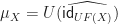
Multiplication: The multiplication is a flattening operation on nested equivalence classes. Formally, $\mu_X = U( \widehat{\mathsf{id}_{UF(X)}})$ .

The multiplication is probably easier to follow from an example.

Example: Returning to the equational presentation of monoids above, an example of the multiplication would be $\mu([w + [y + z] ]) = [w + (y + z)]$ .

Any choice of operations and equations then produces a monad on the category $\mathsf{Set}$ , yielding boundless examples.

Example: There are monads on $\mathsf{Set}$ induced by the equational presentations of monoids, commutative monoids, groups, Abelian groups, rings, join semilattices, semigroups…

The monads that arise from equational presentations are known as the finitary monads. We may return to the question of exactly what that means in a future post. Possibly more important to note is that if we consider sufficiently liberal generalizations of the arities in our equational presentations, every $\mathsf{Set}$ monad can be described in such a way.