stringdiagram

An application of monadicity

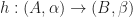
Now we have seen the basic ideas of monadicity, and Beck’s monadicity theorem, it’s time to look at an important application. Although the result in question belongs to the area of topos theory, to avoid pulling in too much additional theory we will consider a concrete example, and then sketch how this extends to the abstract setting.

Subsets and the contravariant powerset

For our motivating example, we are going to consider the category $\mathsf{Set}$ of sets and functions. The set

$\{ \mathsf{true}, \mathsf{false} \}$

which we shall denote $2$ will play an important role. For any set $X$ , a function $\chi : X \rightarrow 2$ corresponds to a subset of $X$ :

$\{ x \mid x \in X \;\text{and}\; \chi(x) = \mathsf{true} \}$

and given any subset $U \subseteq X$ , we can define a function:

$x \mapsto \begin{cases} \mathsf{true} & \text{ if } x \in U \\ \mathsf{false} & \text{otherwise} \end{cases}$

In this way, we can go back and forth between subsets and what are known as their characteristic functions. For a fixed set $X$ , we can consider the set $2^X$ of characteristic functions of subsets of $X$ . The mapping

$X \mapsto 2^X$

extends to a functor. For $f : X \rightarrow Y$ we get a function in the opposite direction $2^f : 2^Y \rightarrow 2^X$ with action:

$\chi \mapsto \chi \circ f$

It is straightforward to check that this satisfies the functor axioms, so we have a functor:

$2^{(-)} : \mathsf{Set}^{op} \rightarrow \mathsf{Set}$ ,

sometimes referred to as the contravariant powerset functor. This functor has a left adjoint, which we shall also denote

$2^{(-)} : \mathsf{Set} \rightarrow \mathsf{Set}^{op}$ .

Notice the only difference here is whether we choose to put the “op” on the domain or codomain. Establishing that these two functors form an adjunction is straightforward, as we have natural bijections between:

Functions $2^X \rightarrow Y$ in $\mathsf{Set}^{op}$
Functions $Y \rightarrow 2^X$ in $\mathsf{Set}$
Functions $Y \times X \rightarrow 2$ in $\mathsf{Set}$
Functions $X \times Y \rightarrow 2$ in $\mathsf{Set}$
Functions $X \rightarrow 2^Y$ in $\mathsf{Set}$

We have seen a more abstract version of this proof before, as this is a special case of the adjunction that induces the continuation monad, in this case for the endofunctor:

$2^{2^{(-)}} : \mathsf{Set} \rightarrow \mathsf{Set}$

The perhaps surprising observation is that the functor

$2^{(-)} : \mathsf{Set}^{op} \rightarrow \mathsf{Set}$

is monadic, meaning the Eilenberg-Moore category of $2^{2^{(-)}}$ is equivalent to $\mathsf{Set}^{op}$ . Put another way, $\mathsf{Set}^{op}$ is monadic over $\mathsf{Set}$ . Aside from being a rather startling fact, this gives a concrete description of the Eilenberg-Moore category of this special case of the continuation monad. Some duality theory tells us that the category of complete atomic Boolean algebras is equivalent to $\mathsf{Set}^{op}$ , and this gives us an even more concrete description of the algebras of this monad.

Generalising

At first glance, the argument above looks very specific to the category of sets and functions. Fortunately, there is a very large class of categories that look sufficiently like the category of sets to carry out this argument in the abstract.

As a first step, we look at the important role of the set $2$ . It allowed us to connect subsets and characteristic functions. To generalise this, we first adopt a more categorical perspective, and consider subobjects rather than subsets. A subobject of object $X$ , is isomorphism class of monomorphisms $U \rightarrowtail X$ . Spelling this out a bit more, two monomorphisms $m : U \rightarrowtail X$ and $m' : U' \rightarrowtail X$ are isomorphic if there exists an isomorphism $i : U \rightarrow U'$ such that $m = m' \circ i$ .

A subobject classifier is a categorical abstraction of the correspondence between subsets (subobjects) and characteristic morphisms. Writing $\mathsf{Sub}(X)$ for the collection of subobjects of $X$ , a category $\mathcal{C}$ with finite limits is said to have a subject classifier if and only if there is an object $\Omega$ and natural isomorphism:

$\mathsf{Sub}(X) \cong \mathcal{C}(X,\Omega)$

There are several equivalent definitions of subobject classifiers. The typical statement involves a generic subobject and a pullback condition, but as we won’t delve into the details, the statement above emphasises the relationship between subobjects and classifying morphisms.

Example: The set $2$ is the subobject classifier in $\mathsf{Set}$ . Subobjects correspond to subsets which correspond to characteristic functions.

The class of categories that look sufficiently like the category of sets for our purposes are known as toposes. A topos is a finitely complete, Cartesian closed category with a subobject classifier. (There are almost as many equivalent definitions of a topos as there are books on the subject, depending on the perspective the author wishes to emphasize. We choose this one as it is reasonably straightforward.). There are many examples of toposes that crop up in mathematical practice.

Example: The category $\mathsf{Set}$ is a topos, and in many ways the motivating example for the abstraction. The full subcategory of finite sets is also a topos.

Example: For any small category $\mathcal{C}$ , the category of presheaves over $\mathcal{C}$ is a topos. This is simply the category with objects functors $\mathcal{C}^{op} \rightarrow \mathsf{Set}$ and morphisms natural transformations between them. This construction can be generalised greatly to various notions of categories of sheaves, but we avoid entering into what would be a sizeable technical detour.

For a topos $\mathcal{C}$ , by analogy with the set theoretic situation, as we have exponentials and a subobject classifier, it is natural to consider the functor:

$\Omega^{(-)} : \mathcal{C}^{op} \rightarrow \mathcal{C}$

It is a non-trivial observation that this functor is monadic. As a concrete argument is no longer possible, this is typically established using a monadicity theorem. Interested readers that are prepared for a bit of topos theory can find the details in any good book on topos theory. Slightly confusingly, topos theorists also refer to this result as the (topos theoretic) monadicity theorem.

This result has an immediate pay-off. As a topos is finitely complete, $\mathcal{C}^{op}$ is also finitely complete. In other words, $\mathcal{C}$ is finitely cocomplete. Finite cocompleteness was actually included in the original definition of a topos, until it was shown that it followed from the other axioms. Monadicity is a particularly elegant way of establishing this fact.

Conclusion

Our discussion of topos theory has been deliberately somewhat sketchy, to avoid pulling in too many technical details. Topos theory is a vast subject, with connections to many parts of mathematics, and would probably warrant a blog of its own.

Further reading: Readers interested in filling in some of the topos theoretic technical details could look at one of the standard sources, such as volume 1 of Johnstone’s “Sketches of an Elephant”, Moerdijk and MacLane’s “Sheaves in Geometry and Logic” or volume 3 of Borceux’s “Handbook of Categorical Algebra”.

A monad is just a one object enriched category

We have seen that the notion of monad can be interpreted in any bicategory. The aim of todays post is to explain that for a bicategory $\mathcal{W}$ , a monad in $\mathcal{W}$ is the same thing as a one-object $\mathcal{W}$ -enriched category. Or more tersely:

A monad is the same thing as a one-object $\mathcal{W}$ -category.

Mostly, this is just a case of understanding the definitions, with no complicated translation between the two structures required.

Monads and enrichment

Recall that for a monoidal category $(\mathcal{V}, \otimes, I)$ , a $\mathcal{V}$ –enriched category, or $\mathcal{V}$ -category $\mathcal{A}$ is a generalisation of ordinary categories with:

A collection of objects $X,Y,\ldots$ .
For every pair of object $X,Y$ , a hom object $\mathcal{A}(X,Y)$ .
For each object $X$ , an identity $\mathcal{V}$ -morphism $j_X : I \rightarrow \mathcal{A}(X,X)$ .
For each triple of objects $X,Y,Z$ , a composition $\mathcal{V}$ -morphism $m_{X,Y,Z} : \mathcal{A}(Y,Z) \otimes \mathcal{A}(X,Y) \rightarrow \mathcal{A}(X,Z)$ .

These are subject to some natural axioms such that composition is associative, and unital with respect to the chosen identities. The motivating special case is that a $\mathsf{Set}$ -enriched category is the same thing as an ordinary category.

It is a well-known fact of enriched category theory that a monoid in the monoidal category $\mathcal{V}$ is the same thing as a one object $\mathcal{V}$ -category. The even better known special case, which crops up in most introductions to category theory, is that a one object ordinary category is the same thing as a monoid.

Of course, the special case that we should be interested in as monad theorists is the monoidal category of endofunctors $([\mathcal{C}, \mathcal{C}], \circ, \mathsf{Id}_{\mathcal{C}})$ . Using the fundamental meme of monad theory, that a monad is just a monoid in the category of endofunctors, we can deduce that monads on $\mathcal{C}$ are the same thing as one object $[\mathcal{C},\mathcal{C}]$ -enriched categories. This claim works equally well if we consider monads in an arbitrary bicategory.

Example: We have seen previously that for a monoidal category $\mathcal{V}$ with coproducts, a $\mathcal{V}$ -enriched category is the same thing as a monad in the bicategory of $\mathcal{V}$ -matrices, $\mathbf{Mat}(\mathcal{V})$ . Applying the observation above, the following all describe the same data:

A $\mathcal{V}$ -enriched category with set of objects $O$ .
A monad on $O$ in $\mathbf{Mat}(\mathcal{V})$ .
A one-object $\mathbf{Mat}(\mathcal{V})(O,O)$ -enriched category.

Which is a bit of a funny conclusion, every multi-object enriched category is the same thing as a single-object enriched category over a different base. In particular, every ordinary (small) category with set of objects $O$ is a one-object $\mathbf{Mat}(\mathsf{Set})(O,O)$ -enriched category.

In the example above, it feels a bit clumsy to have to keep saying “…with set of objects $O$ …”. To clean this up, and take this story a bit further, we are going to have to generalise our notion of enriched category, to categories enriched over a bicategory $\mathcal{W}$ . Although this may sound a bit intimidating, it is actually only a small step beyond enrichment in a monoidal category.

A $\mathcal{W}$ -enriched category $\mathcal{A}$ consists of:

A collection of objects $X,Y,Z$ , each with an associated extent, given by a 0-cell $\mathsf{ext}(X)$ in $\mathcal{W}$ .
For every pair of objects $X,Y$ , a hom 1-cell $\mathcal{A}(X,Y) : \mathsf{ext}(X) \rightarrow \mathsf{ext}(Y)$ .
For every object $X$ , an identity 2-cell $j_A : \mathsf{Id}_{\mathsf{ext}(X)} \Rightarrow \mathcal{A}(X,X)$ .
For every triple of objects $X,Y,Z$ , a composition 2-cell $m_{X,Y,Z} : \mathcal{A}(Y,Z) \circ \mathcal{A}(X,Y) \Rightarrow \mathcal{A}(X,Z)$ .

As before, this data is subject to natural unitality and associativity axioms.

With this definition in place, naming things suggestively, a one object $\mathcal{W}$ -category consists of:

An object, with extent a 0-cell $\mathcal{C}$ in $\mathcal{W}$ .
A single hom 1-cell $\mathbb{T} : \mathcal{C} \rightarrow \mathcal{C}$ .
An identity 2-cell $\eta : \mathsf{Id} \Rightarrow \mathbb{T}$ .
A single composition 2-cell $\mu : \mathbb{T} \circ \mathbb{T} \Rightarrow \mathbb{T}$ .

This data satisfies exactly the axioms such that $(\mathbb{T} : \mathcal{C} \rightarrow \mathcal{C}, \eta, \mu)$ is a monad. That is:

A monad in $\mathcal{W}$ is the same thing as a one-object $\mathcal{W}$ -category.

We rephrase the previous example in this more flexible setting.

Example: For a monoidal category $\mathcal{V}$ , a $\mathcal{V}$ -category is a one object $\mathbf{Mat}(\mathcal{V})$ -enriched category.

A possibly more interesting example is as follows.

Example: We have seen previously that for a category $\mathcal{C}$ with pullbacks, an internal category in $\mathcal{C}$ is the same thing as a monad in the bicategory of spans $\mathbf{Span}(\mathcal{C})$ . Now applying our previous observation, the following all describe the same data:

An internal category in $\mathcal{C}$ .
A monad in $\mathbf{Span}(\mathcal{C})$ .
A one-object $\mathbf{Span}(\mathcal{C})$ -enriched category.

This establishes a slightly surprising connection between internal and enriched category theory.

Conclusion

To an extent, this post is about almost trivial relationships between definitions that happen to coincide. This is not just an exercise in categorical showing-off or pointless abstraction. The relationship between monads and one-object enriched categories is really a matter of perspective. This may allow us to relate monads to other concepts, for example finitary monads and Lawvere theories can be connected in this way. Once monads are viewed as categories, we can consider categorical notions such as completion under certain limits or colimits, which again occur in connection with Lawvere theories. These ideas are used to startling effect in the work of Richard Garner and co-authors, which I highly recommend as further reading.

Algebras are regular quotients of free algebras

The aim of this post is to show that for a monad

$(\mathbb{T} : \mathcal{C} \rightarrow \mathcal{C}, \eta : \mathsf{Id}_{\mathcal{C}} \Rightarrow \mathbb{T}, \mu : \mathbb{T}^2 \Rightarrow \mathbb{T})$ ,

every Eilenberg-Moore algebra $(A,\alpha : \mathbb{T}(A) \rightarrow A)$ is given as the coequalizer of a parallel pair of morphisms between free algebras in $\mathcal{C}^{\mathbb{T}}$ . In this case, we say that $(A,\alpha)$ is a regular quotient of free algebras. Notice we are not making any any assumptions about the base category $\mathcal{C}$ such as (co)completeness, so we don’t have a lot to work with. Really the only available structure is:

The unit and multiplication of the monad, and the axioms they satisfy.
The two axioms that every Eilenberg-Moore algebra satisfies relating its structure map to the unit and multiplication.

So we have a handful of morphisms, and some equations that they satisfy, and that’s it. Let’s have a look at how this magic trick is performed.

A parallel pair of algebra morphisms

As a first step, we note that for an Eilenberg-Moore algebra $(A,\alpha)$ , we have a parallel pair of $\mathcal{C}^{\mathbb{T}}$ morphisms:

$\mu_A, \mathbb{T}(\alpha) : F^{\mathbb{T}}(\mathbb{T}(A)) \rightarrow F^{\mathbb{T}}(A)$

Expanding the action of the free algebra functor, this is a pair of morphisms:

$\mu_A, \mathbb{T}(\alpha) : (\mathbb{T}^2(A), \mu_{\mathbb{T}^2(A)}) \rightarrow (\mathbb{T}(A), \mu_A)$

That $\mu_A$ is an algebra morphism is equivalent to the Eilenberg-Moore algebra multiplication axiom. That $\mathbb{T}(\alpha)$ is an algebra morphism is simply naturality of the monad multiplication.

By naturality of $\mu$ , we note that there is an algebra morphism in the opposite direction:

$\mathbb{T}(\eta_A) : (\mathbb{T}(A), \mu_A) \rightarrow (\mathbb{T}^2(A), \mu_{\mathbb{T}^2(A)})$

Furthermore, by the monad right unitality axiom

$\mu_A \cdot \mathbb{T}(\eta_A) = \mathsf{id}_{\mathbb{T}(A)}$

and by the algebra unit axiom:

$\mathbb{T}(\alpha) \cdot \mathbb{T}(\eta_A) = \mathsf{id}_{\mathbb{T}(A)}$

Therefore these three morphisms form a reflexive pair.

A coequalizer in the base category

We now apply the forgetful functor $U^{\mathbb{T}} : \mathcal{C}^{\mathbb{T}} \rightarrow \mathcal{C}$ , yielding a parallel pair.

$U^{\mathbb{T}}(\mu_A), U^{\mathbb{T}}(\mathbb{T}(\alpha)) : U^{\mathbb{T}} \circ F^{\mathbb{T}}(\mathbb{T}(A)) \rightarrow U^{\mathbb{T}}(\alpha) : U^{\mathbb{T}} \circ F^{\mathbb{T}}(A)$

which if we unpack the definitions is simply a parallel pair of $\mathcal{C}$ -morphisms:

$\mu_A, \mathbb{T}(\alpha) : \mathbb{T}^2(A) \rightarrow \mathbb{T}(A)$

Our current aim is to find a coequalizer of this pair, knowing it must have codomain $A$ . The obvious choice is to consider

$\alpha : \mathbb{T}(A) \rightarrow A$

as our candidate universal coequalizer morphism. By the algebra multiplication axiom, we have

$\alpha \cdot \mu_A = \alpha \cdot \mathbb{T}(\alpha)$

which is an encouraging first step to establishing this forms a coequalizer diagram. To establish the universal property, we are going to need a bit more. Using components of the monad unit, we get two other useful $\mathcal{C}$ -morphisms:

$\eta_A : A \rightarrow \mathbb{T}(A)$ .
$\eta_{\mathbb{T}(A)} : \mathbb{T}(A) \rightarrow \mathbb{T}^2(A)$ .

By the algebra unit axiom

$\alpha \cdot \eta_A = \mathsf{id}_A$

and by the monad left unitality axiom

$\mu_A \cdot \eta_{\mathbb{T}(A)} = \mathsf{id}_{\mathbb{T}(A)}$

Finally, by naturality:

$\mathbb{T}(\alpha) \cdot \eta_{\mathbb{T}(A)} = \eta_A \cdot \alpha$ .

We have shown the our parallel pair form a contractible coequalizer in the base category, and further that the parallel pair of algebra morphism:

$\mu_A, \alpha : F^{\mathbb{T}}(\mathbb{T}(A)) \rightarrow F^{\mathbb{T}}(A)$

form a reflexive $U^{\mathbb{T}}$ -contractible pair.

An algebra coequalizer

We would now like to conclude we have a coequalizer in the Eilenberg-Moore category. Recall that the forgetful functor $U^{\mathbb{T}} : \mathcal{C}^{\mathbb{T}} \rightarrow \mathcal{C}$ creates colimits that are preserved by $\mathbb{T}$ and $\mathbb{T}^2$ . As contractible coequalizers are absolute colimits, we can apply this result to lift the coequalizer to the Eilenberg-Moore category.

Finally, we note that $\alpha$ is in fact an algebra morphism of type:

$F^{\mathbb{T}}(A) \rightarrow (A,\alpha)$

by the Eilenberg-Moore algebra multiplication axiom. Therefore

$F^{\mathbb{T}}(\mathbb{T}(A)) \xrightarrow{ \mu_A, \alpha} F^{\mathbb{T}}(A) \xrightarrow{\alpha} (A,\alpha)$

is a coequalizer diagram in the Eilenberg-Moore category, and $(A,\alpha)$ is a regular quotient of free algebras as claimed.

Conclusion

We encountered reflexive $U$ -contractible coequalizers in the statement of Beck’s monadicity theorem. In this post, we have seen one example of why these particular absolute colimits are important in the theory of monads, as they can be used to construct every Eilenberg-Moore algebra as a quotient of a free algebra.

Proving this result from very few assumptions, beyond some morphisms satisfying certain equations, leads us to the construction of coequalizers which are defined by by equations between morphisms. Such constructions are necessary absolute, and this at least partially explains the significance of absolute colimits in this context.

Beck’s Monadicity Theorem

Now we have introduced the idea of monadicity, we move onto the most important theorem in this area. Beck’s monadicity theorem tells us that a functor $U: \mathcal{B} \rightarrow \mathcal{C}$ is monadic if and only if the following three conditions hold:

U has a left adjoint.
U reflects isomorphisms.
$\mathcal{B}$ has coequalizers of reflexive $U$ -contractible pairs, and $U$ preserves them.

The aim of this post is to unpack these three conditions, and to justify why they are at least necessary for a monadic functor. That they are also sufficient is a rather amazing fact that we may delve into in another post. The first two conditions are relatively trivial, but the third will require more consideration.

Left adjoints

The first condition, that $U$ has a left adjoint is the most trivial. By definition, we require a monadic functor to be a right adjoint so we can consider the comparison functor to the Eilenberg-Moore category.

Isomorphism reflection

A functor $U$ is said to reflect isomorphisms, or to be conservative, if for every $f$ , $U(f)$ is an isomorphism implies $f$ is.

Remark: Isomorphism reflection is a statement about morphisms not objects. It does not say that if $U(A)$ is isomorphic to $U(B)$ then $A$ is isomorphic to $B$ .

For a monad $\mathbb{T} : \mathcal{C} \rightarrow \mathcal{C}$ , if we have an Eilenberg-Moore algebra morphism $h : (A,\alpha) \rightarrow (B,\beta)$ , then in $\mathcal{C}$

$h \cdot \alpha = \beta \cdot \mathbb{T}(h)$ .

Now assume there exists $\mathcal{C}$ -morphism $g : B \rightarrow A$ such that

$g \cdot h = \mathsf{id}_{A}$ and $h \cdot g = \mathsf{id}_{B}$

then we would like to show $g$ is an algebra morphism of type $(B,\beta) \rightarrow (A,\alpha)$ . This is a straightforward calculation:

$g \cdot \beta = g \cdot \beta \cdot \mathbb{T}(h \cdot g) = g \cdot h \cdot \alpha \cdot \mathbb{T}(g) = \alpha \cdot \mathbb{T}(g)$ .

Therefore $U^{\mathbb{T}}$ reflects isomorphisms. It is easy to verify that equivalences are also conservative, and conservative functors are closed under composition. As

$U = U^{\mathbb{T}} \circ K$

where $K$ is the comparison functor, if $U$ is monadic, it must be conservative. This condition is already sufficient to weed out various putative monadic functors.

Example: Let $\mathsf{Pos}$ be the category of posets and monotone maps, and $U : \mathsf{Pos} \rightarrow \mathsf{Set}$ the obvious forgetful functor. This functor has a left adjoint, and so satisfies the first condition of the monadicity theorem. Now consider the two element posets:

The poset $X$ , with underlying set $\{ x_1, x_2 \}$ with the discrete partial order.
The poset $Y$ , with underlying set $\{ y_1, y_2 \}$ with the least partial order such that $y_1 \leq y_2$ .

There is a bijective monotone map $h : X \rightarrow Y$ with $h(x_1) = y_1$ and $h(x_2) = y_2$ . This morphism has no inverse monotone map. On the other hand, the underlying function $U(h)$ has an obvious inverse in $\mathsf{Set}$ . Therefore $U$ is not conservative, and therefore cannot be monadic.

This argument is easily adapted to show the forgetful functor $\mathsf{Cat} \rightarrow \mathsf{Set}$ taking a small category to its set of objects is not monadic.

The coequalizer condition

We now need to untangle the final condition, and this will be a little bit more technical. We need to introduce two related notions.

Firstly, a parallel pair:

$d^0, d^1 : A \rightarrow B$

is said to be contractible (or split) if there exists $t : B \rightarrow A$ such that

$d^0 \cdot t = \mathsf{id}_B$ and $d^1 \cdot t \cdot d^0 = d^1 \cdot t \cdot d^1$ .

Notice that these conditions are asymmetrical in $d^0$ and $d^1$ .

Secondly, a contractible (or split) coequalizer consists of the following data:

A parallel pair $d^0, d^1 : A \rightarrow B$ .
A morphism $t : B \rightarrow A$ .
A morphism $d : B \rightarrow C$ .
A morphism $s : C \rightarrow B$ .

such that:

$d$ coequalizes the parallel pair, that is $d \cdot d^0 = d \cdot d^1$ .
$d^0$ has section $t$ , that is $d^0 \cdot t = \mathsf{id}_B$ .
$d$ has section $s$ , that is $d \cdot s = \mathsf{id}_C$ .
$d^1 \cdot t = s \cdot d$ .

Again, notice the asymmetry of the conditions. As suggested by the terminology, a contractible coequalizer is a coequalizer in the ordinary sense.

Furthermore, a contractible coequalizer is simply a collection of morphisms satisfying four equations. If we apply a functor to the morphisms, the resulting data will also satisfy the same equations, as functors preserve them, and will therefore also form a contractible coequalizer. Therefore contractible coequalizers are preserved by every functor. That is, they are an example of an absolute colimit.

A second useful fact, connecting these two notions, is that if a contractible pair $d^0, d^1 : A \rightarrow B$ has a coequalizer $d : B \rightarrow C$ , then there automatically exists an $s : C \rightarrow B$ such that it forms a contractible coequalizer.

A $U$ -contractible pair, is a pair $d^0, d^1 : A \rightarrow B$ such that $U(d^0), U(d^1) : U(A) \rightarrow U(B)$ has a contractible coequalizer. Notice this terminology is slightly misleading, we are requiring a contractible coequalizer, not just a contractible pair.

With that mass of terminology in place, we recall that for any monad $\mathbb{T}$ , the forgetful functor $U^{\mathbb{T}} : \mathcal{C}^{\mathbb{T}} \rightarrow \mathcal{C}$ creates colimits which exist in the base category and are preserved by $\mathbb{T}$ and $\mathbb{T}^2$ . $U$ -contractible pairs induce absolute coequalizers in the base category, which are therefore created by $U^{\mathbb{T}}$ . Secondly, although equivalences don’t necessarily create colimits that exist, they do preserve them. Therefore, if $U : \mathcal{B} \rightarrow \mathcal{C}$ is monadic, as

$U = U^{\mathbb{T}} \circ K$

$\mathcal{B}$ has coequalizers of $U$ -contractible pairs, and $U$ preserves them.

In fact, this is stronger than the proof of the monadicity theorem needs, and we can restrict our attention to a small class of coequalizers. A parallel pair $d^0, d^1 : A \rightarrow B$ is said to be reflexive if they have common section. That is, there exists an $r : B \rightarrow A$ such that

$d^0 \cdot r = \mathsf{id}_B = d^1 \cdot r$ .

Conclusion

Two out of the three conditions of the monadicity theorem are pretty routine. The third took a bit of unravelling, but enduring the technicalities is a worthwhile investment, as these special colimits arise again and again in the theory of monads. We will look in detail at the most important source of these special coequalizers in a later post.

Further reading: Our account owes a lot to that of Barr and Well’s in Toposes Triples and Theories. We have deliberately used similar notational choices to them in case readers want to consult their work for further details, which is highly recommended. Johnstone remarks in the Elephant that the restriction to reflexive pairs in condition three is omitted in many accounts, but is all that is needed. Toposes, Triples and Theories is also careful in this regard.

The Idea of Monadicity

Naively, for a given category $\mathcal{B}$ , we might wonder if it is equivalent to the Eilenberg-Moore category of a monad. This would help us deduce properties of $\mathcal{B}$ , such as (co)completeness, using facts we know about the Eilenberg-Moore construction.

Giving this a moments thought, it doesn’t sound quite right, as to deduce properties of an Eilenberg-Moore category, we need more information, for example about the base category. In order to reach a mathematically useful notion, we need to pin down exactly what we intend with regard to this equivalence.

We would like to know what the base category we’re interested in is, and how it relates to $\mathcal{B}$ , so it is natural to consider functors of the form.

$U : \mathcal{B} \rightarrow \mathcal{C}$

Intuitively this is a candidate forgetful functor from an Eilenberg-Moore category to its base category. If there is any hope of $\mathcal{B}$ being equivalent to an Eilenberg-Moore category, $U$ should have a left adjoint

$F : \mathcal{C} \rightarrow \mathcal{B}$ .

This gives us a bit more to work with, as adjunction will give us a monad

$\mathbb{T} = U \circ F$

We are now interested in when there is an equivalence:

$\mathcal{B} \simeq \mathcal{C}^{\mathbb{T}}$

To specify this equivalence more precisely, recall we have already seen the Eilenberg-Moore comparison functor, which relates resolutions of the same monad. Recall this is the unique functor

$K : \mathcal{B} \rightarrow \mathcal{C}^{\mathbb{T}}$

that commutes with the free and forgetful functors, in that:

$U^{\mathbb{T}} \circ K = U$ and $K \circ F = F^{\mathbb{T}}$ .

We have now arrived at the right notion. A right adjoint functor $U : \mathcal{B} \rightarrow \mathcal{C}$ is monadic if the comparison functor is an equivalence of categories. If there exist such a $U$ , we say that $\mathcal{B}$ is monadic over $\mathcal{C}$ .

Monadicity Theorems

Unsurprisingly, a monadicity theorem gives conditions under which a functor is monadic. The key result is known as Beck’s monadicity theorem, which gives precise conditions for monadicity. There are many variations, often with sufficient assumptions that are more convenient to establish in practice. There are also a family of related results, which don’t specifically establish monadicity, but rather other nice properties of the comparison functor.

In fact, if you have a specific functor with a left adjoint, it is often easier to establish monadicity by directly proving the required equivalence. So what’s the point of monadicity theorems? Their main application is when you are working more abstractly, aiming to show that under suitable assumptions that all functors of a certain type are monadic. This situation is similar to the use of adjoint functor theorems. Again, these are rarely applied to establish that a particular functor has an adjoint, but rather that in an abstract setting every functor satisfying certain axioms always has an adjoint.

In our discussions, we will focus on when the comparison functor is an equivalence. MacLane considers the stronger situation where the comparison functor is an isomorphism. We will pay this perhaps less categorically natural formulation less attention. It is however important to be aware that there are monadicity theorems of this type as well when looking at the wider literature.

If instead of the Eilenberg-Moore construction, we consider the Kleisli construction, we can ask similar questions. The situation is much simpler in this case, as was previously discussed.

Conclusion

The notions of monadicity and monadicity theorems are fundamental tools. Despite this, as they are used in more abstract work, they tend to be perceived as a more advanced topic. This is probably reinforced by the fact that the details of monadicity theorems are a little bit technical looking, with certain special classes of colimits having a prominent role. In reality, the details only involve elementary ideas, and are not particularly challenging. We will discuss the specifics of monadicity theorems, related results about comparison functors, and their applications in future posts.

Eilenberg-Moore limits and colimits

For every monad $\mathbb{T} : \mathcal{C} \rightarrow \mathcal{C}$ , we have seen that the Eilenberg-Moore construction yields a new category $\mathcal{C}^{\mathbb{T}}$ . So far, we don’t have a lot of general facts about Eilenberg-Moore categories we can exploit. In fact, these categories are typically very nice, with lots of good properties that a category theorist might hope for being inherited from their base categories. In this post, we will consider (co)completeness of Eilenberg-Moore categories.

Creation of limits and colimits

A functor

$U : \mathcal{A} \rightarrow \mathcal{B}$

is said to create limits of shape $\mathcal{D}$ if for every diagram

$D : \mathcal{D} \rightarrow \mathcal{A}$

the limit $\lim_{U \circ D}$ exists, with limit cone:

$\lim_{U \circ D} \xrightarrow{\lambda_I} UD(I)$

and there exists a unique $D$ -cone

$L \xrightarrow{\lambda'_I} D(I)$

living above the limit cone, that is for all $I$

$U(\lambda'_I) = \lambda_I$

Furthermore, $(L, \lambda')$ is the limit of the diagram $D$ .

The point of knowing that a functor creates limits is that assuming we understand those limits in the codomain category, we the know both:

Limits of the same shape exist in the domain category.
We can explicitly calculate those limits from those in the base category.

There is an obvious dual notion of a functor that creates colimits.

Limits in Eilenberg-Moore Categories

For a monad $\mathbb{T}$ , recall that there is a forgetful functor:

$U^{\mathbb{T}} : \mathcal{C}^{\mathbb{T}} \rightarrow \mathcal{C}$

We have seen that this functor has a left adjoint, and so will preserve all limits that exist in $\mathcal{C}^{\mathbb{T}}$ for standard reasons. It turns out, we can say a lot more than that. In fact $U^{\mathbb{T}}$ creates all limits that exist in $\mathcal{C}$ .

Lets look at what this means in more detail. The action of $U^{\mathbb{T}}$ on algebra morphisms is trivial:

$U^{\mathbb{T}}(h) = h$

Therefore, for diagram:

$D : \mathcal{D} \rightarrow \mathcal{C}^{\mathbb{T}}$

if $\lim_{U^{\mathbb{T}} \circ D}$ exists, with limit cone:

$\lim_{U^{\mathbb{T}} \circ D} \xrightarrow{\lambda_I} U^{\mathbb{T}}D(I)$

then there exists a unique Eilenberg-Moore algebra structure $\alpha$ on $\lim_{U^{\mathbb{T}} \circ D}$ such that each $\lambda_I$ is an algebra homomorphism:

$(lim_{U^{\mathbb{T}} \circ D}, \alpha) \rightarrow D(I)$

and this is the limit cone in $\mathcal{C}^{\mathbb{T}}$ .

This result is fairly easy to prove. The universal property of the limit of $U^{\mathbb{T}} \circ D$ completely determines what $\alpha$ can be. Verifying it is an Eilenberg-Moore algebra, and satisfies the required universal property in $\mathcal{C}^{\mathbb{T}}$ requires further applications of the universal property of the limit in the base category.

This theorem gives us a very good handle on limits in Eilenberg-Moore categories:

$\mathcal{C}^{\mathbb{T}}$ is as complete as the base category $\mathcal{C}$ .
We can calculate these limits explicitly, using our understanding of limits in the base category.

Colimits in Eilenberg-Moore Categories

The situation for colimits is not as good as that for limits, but it’s still pretty nice. There are standard theorems that address some important cases.

Firstly, $U^{\mathbb{T}}$ creates every colimit which exists in the base category and is preserved by $\mathbb{T}$ and $\mathbb{T} \circ \mathbb{T}$ . Again, we get very nice behaviour, but for a slightly strange looking restricted class of colimits. The proof is similar to that for limits, exploiting the universal property of colimits in the base category to find a unique algebra structure map such that the cocone morphisms in the base category are algebra morphisms. The additional preservation assumptions are used to get colimits of the required shape to complete the argument.

You may ask where we are going to find colimits that satisfy these assumptions. There are special colimits called absolute colimits, which are preserved by every functor. These colimits are important in the theory of monads, particularly what are known as monadicity theorems, which we have only briefly touched upon so far. Applying the result above tells us that $U^{\mathbb{T}}$ creates all absolute colimits which exist in the base category.

If you’re wondering how on earth there can be colimits which are preserved by every functor, or how we might prove such a thing, it is instructive to think about what functors preserve. As functors are homomorphisms of categories, they preserve commuting diagrams. It turns out there are certain limits which are characterised by certain diagrams commuting, and therefore are automatically preserved by every functor. We will discuss concrete examples, specifically certain special classes of coequalizers, in later posts when we look at monadicity theorems in more detail.

Another important results is that $\mathcal{C}^{\mathbb{T}}$ is cocomplete if the base category is, and $\mathcal{C}^{\mathbb{T}}$ has coequalizers. This is because in Eilenberg-Moore categories, we can then construct coproducts using these coequalizers, and that establishes cocompleteness. Using this observation, Linton established that for $\mathsf{Set}$ monads, Eilenberg-Moore categories are cocomplete. Note these results are weaker than those we saw before, as there is no suggestion that these colimits are created by $U^{\mathbb{T}}$ , and so the situation is getting wilder. There are more axiomatic versions of Linton’s result, which can then be applied in settings beyond $\mathsf{Set}$ to establish cocompleteness of Eilenberg-Moore categories.

Conclusion

As a warm up application of the results above, and the connection between monads and universal algebra, we can conclude that:

Categories of algebraic structures such as monoids, groups, rings and so on are all complete and cocomplete.
The limits in these algebraic categories are created by the forgetful functor to $\mathsf{Set}$ .
Certain well behaved colimits in these algebraic categories are also created by the forgetful functor.

We will see some more exciting applications of these results later, once we have discussed some other machinery.

This is only one aspect of the niceness of Eilenberg-Moore categories. There are further tame conditions under which the Eilenberg-Moore category is either regular or locally presentable for example. Certain special classes of monads, such as commutative monads imply further structure on the Eilenberg-Moore category. We shall return to these topics later.

Further reading: The results in this post are all very well known, and can be found in all the standard sources, such as Categories for the Working Mathematician, Toposes, Triples and Theories, or volume 2 of the Handbook of Categorical Algebra.

The Relative Monad Eilenberg-Moore Construction

In previous posts, we have seen that relative adjunctions induce relative monads, and in fact every relative monad arises in this way via a Kleisli construction. The Kleisli construction is the initial adjunction that induces a given relative monad. In this post, we are going to look at an Eilenberg-Moore construction that yields a terminal resolution of every relative monad.

As relative monads are described as a variant of Kleisli triples, this made describing the Kleisli construction very straightforward. Unfortunately, this formulation will make the Eilenberg-Moore construction a little bit fiddlier.

Algebras of a Relative Monad

For a $J : \mathcal{C} \rightarrow \mathcal{D}$ -relative monad $(\mathbb{T},\eta,(-)^*)$ , an Eilenberg-Moore algebra consists of:

A carrier $\mathcal{D}$ -object $A$ .
For every $\mathcal{C}$ -object $X$ and $\mathcal{D}$ -morphism $v : J(X) \rightarrow A$ , a morphism $\alpha(v) : \mathbb{T}(X) \rightarrow A$ .

These must satisfy the following axioms:

For every $\mathcal{C}$ -object $X$ and $v : J(X) \rightarrow A$ , $v = \alpha(v) \cdot \eta_Z$ .
For every pair of $\mathcal{C}$ -objects $X$ and $Y$ , $\mathcal{C}$ -object $s : J(X) \rightarrow \mathbb{T}(Y)$ and $v : J(Y) \rightarrow A$ , $\alpha (\alpha(v) \cdot s) = \alpha(v) \cdot s^*$ .

A morphism of Eilenberg-Moore algebras of type $(A,\alpha) \rightarrow (B, \beta)$ is a $\mathcal{D}$ -morphism $h : A \rightarrow B$ such that for every $\mathcal{D}$ -morphism $v : J(Z) \rightarrow A$ :

$h \cdot \alpha(v) = \beta(h \cdot v)$

These form a category $\mathbf{EM}(\mathbb{T})$ , the Eilenberg-Moore category.

Compared to the definition of the Kleisli category for a relative monad, the Eilenberg-Moore category is rather cumbersome. To get some intuition for what is going on, we will look at a particular example in some detail. As suggested by the term Eilenberg-Moore algebra, we we consider an algebraic example.

Recall that a monoid is a structure with a binary operation, which we will write as $\times$ , and a unit, denoted $1$ , satisfying the following three equations:

Left unit: $1 \times x = x$ .
Right unit: $x \times 1 = x$ .
Associativity: $x \times (y \times z) = (x \times y) \times z$ .

Given a set $X$ , we can form the set of equivalence classes of terms built up from multiplication, the unit and variables. Terms are considered equivalent if they are provably equal in equational logic from the axioms of a monoid. For example

$1, 1 \times x, x \times 1, x \times (1 \times 1), x \times y, \ldots$

are all terms, and the first four are provably equal. Only finitely many variables may appear in any given term, but the collection of equivalence classes of terms over a finite set is infinite. For example, even if we have just one variable $x$ , non of the following terms can be proved equal:

$x, x \times x, x \times (x \times x), x \times (x \times (x \times x)), \ldots$

This suggests we consider the functor $J : \mathsf{FinSet} \rightarrow \mathsf{Set}$ including the finite sets into the infinite sets, relating the finite and infinite aspects at play. For any finite set $X$ , we can then take $\mathbb{T}(X)$ to be the equivalence class of terms over $X$ . There is an obvious function:

$\eta_X : J(X) \rightarrow \mathbb{T}(X)$

picking out the equivalence class of each variable in $J(X)$ . Finally, we can think of a function

$f : J(X) \rightarrow \mathbb{T}(Y)$

as specifying a family of equivalence classes of terms over the set finite $Y$ , indexed by the finite set $X$ . Informally, the extension

$f^* : \mathbb{T}(X) \rightarrow \mathbb{T}(Y)$

is a substitution operation, taking equivalence classes of terms over $X$ to those over $Y$ , replacing variables as specified by $f$ . This data together forms a $J$ -relative monad $(\mathbb{T},\eta,(-)^*)$ .

Remark: The relative monad we have just described is the one induced from the ordinary list monad. This is unsurprising as the list monad is the free monoid monad.

A monoid consists of a carrier set $A$ and a choice of:

A function $\times^A : A \times A \rightarrow A$ telling us how the binary operation behaves.
A constant $1^A \in A$ specifying the value of the unit.

Given a term such as

$x \times y \times 1$

and a monoid $(A, \times^A, 1^A)$ , we can evaluate this term to an element of the carrier using the specified multiplication operation and unit constant, if we are given an element in the carrier for each of the variables. In fact, we should get the same value for any term provably equal to this one such as

$x \times y$

Therefore, for any valuation, $v : J(X) \rightarrow A$ , a monoid allows us to build a function

$\alpha(v) : \mathbb{T}(X) \rightarrow A$

which inductively evaluates terms over the same finite set, using the valuation to assign values to the unknowns. This function has some nice properties. Firstly, if a term is the equivalence class of a variable, it will return the value assigned to that variable. This is captured by the equation:

$\alpha(v) \cdot \eta_X = v$

Secondly, it respects the compositional structure of terms. We can think of a function $s : J(X) \rightarrow \mathbb{T}(Y)$ as specifying a substitution, which allows us to build a “bigger” $\mathbb{T}(Y)$ term from a $\mathbb{T}(X)$ term, by using the substitution to replace all the variables with terms over $Y$ . Our evaluation function $\alpha$ builds up results inductively, so we can either evaluate subterms, and then combine them, or evaluate an entire composite term, and we get the same result. This intuition is encoded in the equation:

$\alpha (\alpha(v) \cdot s) = \alpha(v) \cdot s^*$

From the discussion above, a monoid induces an Eilenberg-Moore algebra. In fact, the two axioms forcing good behaviour in terms of variables and compositional structure mean that every Eilenberg-Moore algebra encodes the structure of a monoid. This is similar to how the good behaviour of the Eilenberg-Moore algebras of an ordinary monad was encoded in the unit and multiplication axioms they are required to satisfying. A bit more work shows that the morphisms in the Eilenberg-Moore category correspond to monoid morphisms, so the Eilenberg-Moore category is actually the category of monoids.

Remark: The Eilenberg-Moore algebras may have infinite carriers, despite the fact the terms and valuations are built up from finite sets of variables.

From this example, our intuitions for an Eilenberg-Moore algebra should be:

The carrier is the carrier of some algebraic object.
The elements of $\mathbb{T}(X)$ can be thought of as terms over some object of variables.
$\alpha(v)$ tells us how to evaluate such terms, with the valuation $v$ specifying the values of the variables.
The axioms specify that the operation $\alpha(v)$ must evaluate terms in an inductive manner, built up from the variables in a compositional manner, using a fixed interpretation for each of the operations.

There is nothing in the above discussion which is specific to monoids. We can choose any algebraic structure presented by finite operations and a set of equations, and the class of models will emerge as the Eilenberg-Moore category of the corresponding $J$ -relative monad.

The Eilenberg-Moore Resolution

For $J : \mathcal{C} \rightarrow \mathcal{D}$ , and $J$ -relative monad $(\mathbb{T},\eta,(-)^*)$ , there is an obvious forgetful functor:

$U^{\mathbb{T}} : \mathbf{EM}(\mathbb{T}) \rightarrow \mathcal{D}$ .

sending an algebra to its carrier. There is also a functor

$F^{\mathbb{T}} : \mathcal{C} \rightarrow \mathbf{EM}(\mathbb{T})$ ,

such that $F^{\mathbb{T}}(X)$ has universe $\mathbb{T}(X)$ , and for $v : J(W) \rightarrow X$ :

$\alpha(v) = v^*$

On morphisms:

$F^{\mathbb{T}}(f) = \mathbb{T}(f)$ .

In fact, $F^{\mathbb{T}}$ is $J$ -relative left adjoint to $U^{\mathbb{T}}$ , and is the terminal resolution of the original relative monad $\mathbb{T}$ .

Conclusion

It is satisfying given the apparently slightly ad-hoc formulation of relative monad that a satisfactory connection with adjunctions emerges. We get two canonical resolutions, the initial Kleisli resolution and the terminal Eilenberg-Moore resolution, exactly as we did in the world of ordinary monad theory.

Our main example was from universal algebra. The relative monad structure allowed us to separate out finitary concerns about variables from infinitary aspects involving the carriers of algebras. This was not directly possible in the ordinary monadic setting, as the restriction to endofunctors forces “all the bookkeeping to happen in the same place”.

Further reading: The Eilenberg-Moore construction is introduced in the original “Monads need not be endofunctors” paper, which as usual is recommended reading.

The Relative Monad Kleisli Construction

We have now seen both relative monads and relative adjunctions, and how every relative adjunction induces a relative monad. As in conventional monad theory, it is natural to ask ourselves if every relative monad arises in this way. The mathematics parallels the situation for ordinary monads. In todays post will look at one extremal construction, generalising the ordinary Kleisli category and its corresponding adjunction.

From a computational perspective, the traditional Kleisli captured the basic aspects of effectful computation. The Kleisli category for a relative monad might be seen as modelling effectful computation on constrained or structured inputs.

Kleisli Categories of Relative Monads

For $J : \mathcal{B} \rightarrow \mathcal{D}$ assume we have a $J$ -relative monad $(\mathbb{T},\eta, (-)^*)$ . The Kleisli category $\mathbf{Kl}(\mathbb{T})$ has:

Objects: The objects of $\mathcal{B}$ .
Morphisms: The morphisms of type $B_1 \rightarrow B_2$ in $\mathbf{Kl}(\mathbb{T})$ are morphisms of type $J(B_1) \rightarrow \mathbb{T}(B_2)$ . The identity at $B$ is $\eta_{B} : J(B) \rightarrow \mathbb{T}(B)$ . The composite $g \bullet f$ in the Kleisli category is given by $g^* \cdot f$ in $\mathcal{D}$ .

The structure of this category, and verifying the category axioms, follow pretty directly from the properties of the Kleisli triple. As with the notion of $J$ -relative monad, the structure of the Kleisli category is a pretty routine generalisation of the ordinary notion, with $J$ inserted in a few places to make things type check.

Remark: We make a different notational choice for the Kleisli category of a relative monad than the one we used in the ordinary situation. This is because the traditional notation seems a bit less natural once the monad is not an endofunctor.

We will now look at a few examples, all arising as the relative monad induced by an ordinary monad, for a suitable choice of $J$ .

Example: Let $J : \mathsf{FinSet} \rightarrow \mathsf{Set}$ be the inclusion of the subcategory of finite sets into the category of sets. The Kleisli category of the $J$ -relative monad induced by the powerset monad $\mathbb{P} : \mathsf{Set} \rightarrow \mathsf{Set}$ is the category with:

Objects: Finite sets
Morphisms: A morphism $A \rightarrow B$ is a binary relation $R \subseteq A \times B$ . Composition and identities are the usual thing for binary relations.

Notice this is neither the Kleisli category of the powerset monad, or the finite powerset monad. In this case, it is equivalent to the powerset monad on the category of finite sets.

In the previous example, everything ended up being finite due to properties specific to the powerset construction. Before we start developing bad intuitions, lets look at a different example that behaves differently.

Example: For $J$ as in the previous example, consider the relative monad induced by the list monad $\mathbb{L}$ . The Kleisli category has:

Objects: Finite sets.
Morphisms: Functions $A \rightarrow \mathbb{L}(B)$ with composition and identities as for the ordinary list monad.

Notice here, this is not the same as the Kleisli category of the list monad itself. There is no obvious analogue of the finite powerset to consider in this case either. Nor can we simply restrict the list monad to an endofunctor on finite sets, as the collection of lists of elements taken from a finite set is infinite. So here we see some genuine interplay between the finite and infinite aspects of the construction.

Another natural, if a bit pathological, source of examples will help to test our intuitions even further.

Example: For any $J : \mathcal{B} \rightarrow \mathcal{D}$ , we can consider the relative monad induced by the identity monad. This will have:

Objects: Objects in the category $\mathcal{B}$ .
Morphisms: Morphisms of type $B_1 \rightarrow B_2$ are $\mathcal{D}$ -morphisms of type $J(B_1) \rightarrow J(B_2)$ . Composition and identities are exactly as in $\mathcal{D}$ .

For different choices of $J$ :

$(-) + 1 : \mathsf{Set} \rightarrow \mathsf{Set}$ gives the category of non-empty sets and functions between them.
$(-) + E : \mathsf{Set} \rightarrow \mathsf{Set}$ gives the category of sets with at least $|E|$ elements, and functions between them.
$(-) \times S : \mathsf{Set} \rightarrow \mathsf{Set}$ has Kleisli category equivalent to the Kleisli category of the state monad with state set $S$ .
$K^{(-)} : \mathsf{Set}^{op} \rightarrow \mathsf{Set}$ has Kleisli category equivalent to the Kleisli category of the continuation monad on set $K$ .

We also note the following obvious example, establishing the connection with ordinary monads.

Example: As we have previously seen, an $\mathsf{Id}$ -relative monad is the same thing as an ordinary monad. The associated Kleisli construction is also the same as in the case of ordinary monads.

The Kleisli Adjunction

For $J : \mathcal{B} \rightarrow \mathcal{D}$ , and $J$ -relative monad $(\mathbb{T}, \eta, (-)^*)$ , we have the following functors:

$F_{\mathbb{T}} : \mathcal{B} \rightarrow \mathbf{Kl}(\mathbb{T})$ , with $F_{\mathbb{T}}(B) = B$ , and $F_{\mathbb{T}}(h) = \eta_B \cdot J(h)$ .
$U_{\mathbb{T}} : \mathbf{Kl}(\mathbb{T}) \rightarrow \mathcal{D}$ , with $U_{\mathbb{T}}(B) = \mathbb{T}(B)$ and $U_{\mathbb{T}}(h) = h^*$ .

It is a routine exercise to show that $F_{\mathbb{T}}$ is a $J$ -relative left adjoint of $U_{\mathbb{T}}$ , and that this adjunction induces the relative monad $\mathbb{T}$ .

We can form a category with objects resolutions of a fixed $J$ -relative monad. A morphism of resolutions via categories $\mathcal{C}_1$ and $\mathcal{C}_2$ is a functor $H : \mathcal{C}_1 \rightarrow \mathcal{C}_2$ commuting with the left and right adjoints in the obvious way. The Kleisli adjunction is initial in this category. For another resolution with left adjoint $L$ , the unique Kleisli comparison functor is given on objects by $K(B) = L(B)$ and on morphisms $K(h)$ is the transpose of $h$ under the codomain adjunction. As taking transposes is a bijection, this functor is full and faithful.

Generalising the situation for ordinary monads:

The comparison functor is an isomorphism iff $L$ is bijective on objects.
The comparison functor is an equivalence iff $L$ is essentially surjective.

Conclusion

We have seen that every relative monad is induced by an adjunction, via a generalisation of the Kleisli construction for ordinary monads. The resulting Kleisli categories were surprisingly varied, given the extra flexibility that relative monads provide.

Given what we have learned about ordinary monad theory, we should ask ourselves whether there is an analogue of the Eilenberg-Moore construction as well. That is the topic we will address next time.

Futher reading: The Kleisli construction for relative monads appears in “Monads need not be endofunctors”. That the characterisation of adjunctions of Kleisli type generalises to the relative setting appears in Nathanael Arkor’s thesis, where they serve an important role in connection to algebra.

Relative Adjunctions and Density

In the previous post, we encountered relative adjunctions. One curious aspect was that if $L$ is left $J$ -relative adjoint to $R$ :

$R$ determines $L$ up to isomorphism.
$L$ does not necessarily determine $R$ up to isomorphism.

In this post, we’re going to look at this aspect of relative adjunctions in more detail. We will see that we get better behaviour if $J$ is a dense functor. This is an important aspect of relative monad theory, so it is worth seeing it in action.

Adjoints determine each other

As before, we will warm up by considering the non-relative situation, and look at ordinary adjunctions. In that case, if $L \dashv R$ and $L \dashv R'$ , we have natural isomorphisms:

$\mathcal{D}(A, R(B)) \cong \mathcal{C}(L(A),B) \cong \mathcal{D}(A,R'(B))$

Now we calculate:

$[\mathcal{C},\mathcal{D}](F,R) \cong \int_C \mathcal{D}(F(C),R(C)) \cong \int_C \mathcal{D}(F(C),R'(C)) \cong [\mathcal{C},\mathcal{D}](F,R')$

The first and final steps use the following standard natural isomorphism relating natural transformations and ends:

$[C,D](F,G) \cong \int_C \mathcal{C}(F(C),G(C))$

The middle step then simply uses our assumed adjunctions. From our calculated isomorphism, as the Yoneda lemma is full and faithful:

$R \cong R'$ ,

so $L$ determines $R$ up to isomorphism. It is clear that we could use a symmetrical argument to show that $L$ is fully determined by $R$ . For a reader familiar with these “Yoneda style” arguments, this is a very routine proof, with the relationship between natural transformations and ends allowing us to make the connection between functors and their actions.

Relative adjunctions

Now we have seen a proof relating adjoints for ordinary adjunctions, lets see how we can adapt it to the $J$ -relative setting. As relative adjunctions are asymmetrical, there are two aspects to consider.

Firstly, we assume that both $L$ and $L'$ are left $J$ -relative adjoint to $R$ , so we have natural isomorphisms:

$\mathcal{C}(L(A), B) \cong \mathcal{D}(J(A),R(B)) \cong \mathcal{C}(L'(A),B)$

We can actually perform an a very similar calculation to before:

$[\mathcal{B},\mathcal{C}](L,F) \cong \int_B \mathcal{C}(L(B),F(B)) \cong \int_B \mathcal{C}(L'(B),F(B)) \cong [\mathcal{B},\mathcal{C}](L',F)$ ,

and so $L \cong L'$ . So far, so straightforward.

Now lets consider the situation for the right adjoint. We now assume that $L$ is left $J$ -relative adjoint to both $R$ and $R'$ , so we have natural isomorphisms:

$\mathcal{D}(J(A),R(B)) \cong \mathcal{C}(L(A),B) \cong \mathcal{D}(J(A),R'(B))$

We can try and proceed as before, with the first step

$[\mathcal{C},\mathcal{D}](F,R) \cong \int_C \mathcal{D}(F(C),R(C))$ ,

but we immediately become stuck, as the only relationships we have involving the functor $R$ also mention $J$ . To make progress, we need something new.

A functor $J : \mathcal{B} \rightarrow \mathcal{D}$ is said to be dense if the restricted Yoneda embedding

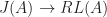
$\mathcal{D} \rightarrow [\mathcal{B}^{op},\mathsf{Set}]$

is full and faithful. Explicitly, this means we have a natural isomorphism:

$\mathcal{D}(D,D') \cong [\mathcal{B}^{op},\mathsf{Set}](\mathcal{D}(J(-),D), \mathcal{D}(J(-),D'))$

This looks encouraging, as $J$ appears exactly in the position we would hope. With the same assumptions as before, assuming $J$ is dense, we calculate:

$\begin{aligned} [\mathcal{C},\mathcal{D}](F,R) &\cong \int_C \mathcal{D}(F(C),R(C)) \\ &\cong \int_C [\mathcal{B}^{op},\mathsf{Set}](\mathcal{D}(J(-),F(C)), \mathcal{D}(J(-),R(C))) \\ &\cong \int_C \int_B \mathsf{Set}(\mathcal{D}(J(B),F(C)), \mathcal{D}(J(B),R(C))) \\ &\cong \int_C \int_B \mathsf{Set}(\mathcal{D}(J(B),F(C)), \mathcal{D}(J(B),R'(C))) \\ &\cong \int_C [\mathcal{B}^{op},\mathsf{Set}](\mathcal{D}(J(-),F(C)), \mathcal{D}(J(-),R'(C))) \\ &\cong \int_C \mathcal{D}(F(C),R'(C)) \\ &\cong [\mathcal{C},\mathcal{D}] (F,R') \end{aligned}$

Therefore, $R \cong R'$ , so if $J$ is dense, right adjoints are determined up to isomorphism.

Conclusion

This post was a bit more technical than usual. This was so that the role of density in the arguments could be made fully explicit. Along the way we saw that density wasn’t a particularly complicated condition, simply allowing us to make Yoneda style arguments in more restrictive settings. Density fits very naturally into calculations involving relative monads or adjunctions, and was introduced by Ulmer in the same paper as relative adjunctions. Ulmer indicates that Gabriel had also introduced the same notion independently at about the same time. Kelly points out in “Basic Concepts in Enriched Category Theory” that the special case of dense subcategories actually goes back further to Isbell’s “Adequate subcategories” from 1960. That the idea has arisen independently several times provides evidence of its utility.

Further reading: I’ve probably recommended it before, but for users wanting more background on these Yoneda style arguments, I strongly recommended Loregian’s “(Co)end calculus” book.

Acknowledgement: Thanks to Nathanael Arkor for very helpful feedback correcting some erroneous remarks relating to the history of dense functors in earlier versions.

Relative Adjunctions

A large part of the richness of ordinary monad theory comes with the interplay between monads and adjunctions. Now we have encountered relative monads, a natural next step is to look for connections with adjunctions. That is the purpose of todays post.

Kleisli Triples and Adjunctions

As relative monads are formulated as a generalisation of Kleisli triples, it makes sense to use the relationship between adjunctions and that formulation of ordinary monads as a starting point, before attempting to generalise to the relative setting.

As we are favouring monads in Kleisli form, it is worth thinking about which formulation of adjunctions is going to fit comfortably. There are many equivalent choices, we can consider adjunctions in terms of:

Cup and cap natural transformations satisfying snake equations.
A pair of functors satisfying a certain unique fill-in condition.
A natural bijection between hom sets $\mathcal{C}(L(A),B) \cong \mathcal{D}(A,R(B))$ .
…

As a monad in Kleisli form has an extension operation:

$(-)^* : \mathcal{C}(A,\mathbb{T}(B)) \rightarrow \mathcal{C}(\mathbb{T}(A),\mathbb{T}(B))$ ,

which is a mapping between hom sets, this seems to connect well with the natural bijection between hom sets formulation of adjunctions. So lets assume we have an adjunction, witnessed by a natural isomorphism:

$\mathcal{C}(L(A),B) \xrightarrow{\theta_{A,B}} \mathcal{D}(A,R(B))$

We wish to show that this induces a monad, using the extension form. The action on objects is:

$X \mapsto RL(X)$

For the unit map, we note that $\theta_{A,L(A)}$ has type

$\mathcal{C}(L(A),L(A)) \xrightarrow{\theta_{A,L(A)}} \mathcal{D}(A,R(L(A)))$

so we take the components of our unit as

$\eta_A = \theta_{A,L(A)}(\mathsf{id})$ .

Finally, we need to identify a suitable extension operation. The following composite has the right type:

$\mathcal{D}(A,RL(B)) \xrightarrow{\theta^{-1}_{A,L(B)}} \mathcal{C}(L(A),L(B)) \xrightarrow{R_{A,B}} \mathcal{D}(RL(A),RL(B))$

where $R_{A,B}$ is the map that applies the functor $R$ to a given hom set. More explicitly, we take:

$f^* = R(\theta^{-1}_{A,B}(f))$ .

We have three axioms to check. Firstly, we calculate:

$\eta^*_A = \theta(\mathsf{id})^* = R(\theta^{-1}(\theta(\mathsf{id})) = R(\mathsf{id}) = \mathsf{id}$ .

Secondly,

$f^* \cdot \eta_A = R(\theta^{-1}(f)) \cdot \theta(\mathsf{id}) =\theta(\theta^{-1}(f) \cdot \mathsf{id}) = \theta(\theta^{-1}(f)) = f$ ,

where we use the naturality of $\theta$ in the only non-trivial step.

Finally:

$g^* \cdot f^* = R(\theta^{-1}(g)) \cdot R(\theta^{-1}(f)) = R(\theta^{-1}(g) \cdot \theta^{-1}(f)) = R(\theta^{-1}(R(\theta^{-1}(g)) \cdot f)) = R(\theta^{-1}(g^* \cdot f) = (g^* \cdot f)^*$

Again, the only non-trivial step uses naturality. With this proof for ordinary monads under our belts, we’re ready to look at relative monads.

Relative adjunctions

We now want to tweak things to try and recover a $J$ -relative monad, from a similar situation to before. Previously, we constructed the unit $\eta_A$ as the image of the identity under a map of type:

$\mathcal{C}(L(A),L(A)) \rightarrow \mathcal{D}(A,RL(A))$

For a $J$ -relative monad, the component of the unit at $A$ has type $J(A) \rightarrow RL(A)$ . This suggests we require a natural isomorphism of type:

$\mathcal{C}(L(A),B) \xrightarrow{\theta_{A,B}} \mathcal{D}(J(A),R(B))$

where $J : \mathcal{J} \rightarrow \mathcal{D}$ , $L : \mathcal{J} \rightarrow \mathcal{C}$ and $R : \mathcal{C} \rightarrow \mathcal{D}$ . If we have such an isomorphism, we can follow an almost identical recipe to before to form a $J$ -relative monad with:

Object map $T(X) = RL(X)$ .
Unit components $\eta_A = \theta(\mathsf{id}) : J(A) \rightarrow RL(A)$ .
Extension operation $f^* = R(\theta^{-1}(f))$ .

The proofs of the three axioms are identical to the previous ones, up to trivial changes in type information.

Our calculations lead us to consider isomorphisms of hom sets of the form:

$\mathcal{C}(L(A),B) \cong \mathcal{D}(J(A),R(B))$

If we have such an natural isomorphism we say that $R$ has a left $J$ -relative adjoint $L$ . We could also consider the situation:

$\mathcal{C}(L(A),J(B)) \cong \mathcal{D}(A,R(B))$

in which case we say that $L$ has a right $J$ -relative adjoint $R$ . Both situations are known as relative adjunctions.

Example: A functor $F : \mathcal{C} \rightarrow \mathcal{D}$ is full and faithful if and only if $\mathsf{Id}$ is its $F$ -relative left adjoint, as that is the case when we have a natural isomorphism:

$\mathcal{C}(A,B) \cong \mathcal{D}(F(A),F(B)$

It follows that every full and faithful functor induces a relative monad.

We also have the obvious source of examples.

Example: Every ordinary adjunction is a $\mathsf{Id}$ -relative adjunction.

We can also build new relative adjoints in a routine way.

Example: If we have relative adjunction:

$\mathcal{C}(L(A),B) \cong \mathcal{D}(J(A),R(B))$

then for any $F$ of appropriate type:

$\mathcal{C}(L(F(A)), B) \cong \mathcal{D}(J(F(A)),R(B))$

so $L \circ F$ is $J \circ F$ -relative left adjoint to $R$ . Using the previous example, given an ordinary adjunction $L \dashv R$ , we get relative adjunctions:

$\mathcal{C}(L(F(A)),B) \cong \mathcal{D}(F(A),R(B))$

so $L \circ F$ is $F$ -relative adjoint to $R$ .

Some words of caution

We have seen that left $J$ -relative adjoints yield $J$ -relative monads. Unfortunately relative adjunctions are not as well behaved as ordinary adjunctions, for example:

The situation is asymmetric. Left $J$ -relative adjoints induce $J$ -relative monads but not comonads, and unit maps of type $J \Rightarrow RL$ , but no counit. On the other hand, right $J$ -relative adjoints induce $J$ -relative comonads but not monads, and counit maps of type $LR \Rightarrow J$ , but no unit.
A functor determines its $J$ -relative left adjoint, but the $J$ -relative left adjoint does not fully determine the right adjoint.
There is an equivalent formulation of relative adjunctions in terms of absolute Kan lifts. This might sound like it would lead to a tidier setting, more suitable for formal category theory. Unfortunately, it does not capture the right notion if we move to the setting of enriched category theory.

Conclusion

By examining the construction of Kleisli triples from ordinary adjunctions, we identified a variation on the notion of adjunction, that induces relative monads. We have seen a small number of examples of relative adjunctions so far. Readers of this blog are probably (hopefully) asking themselves the following questions:

Does every relative monad arise via an adjunction?
Is there a suitable generalisation of the Kleisli construction?
Is there a suitable generation of the Eilenberg-Moore construction?

Positive answers to these questions would provide stronger evidence that relative adjunctions are a reasonable concept. We shall explore these topics in future posts.

Further reading: Ulmers “Properties of Dense and Relative Adjoint Functors” is a good place to start for more background, and is surprisingly readable for an older category theory paper.

Acknowledgements: Nathanael Arkor helpfully pointed out a blunder in an earlier version of this post, where I had muddled up Kan extensions and lifts in a remark.