Distributive Laws

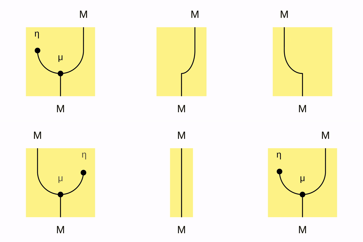
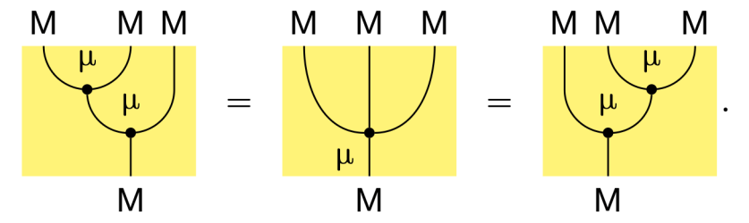
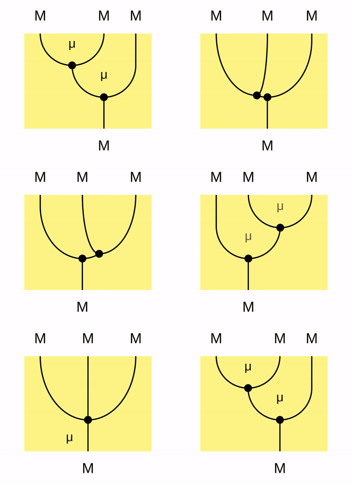
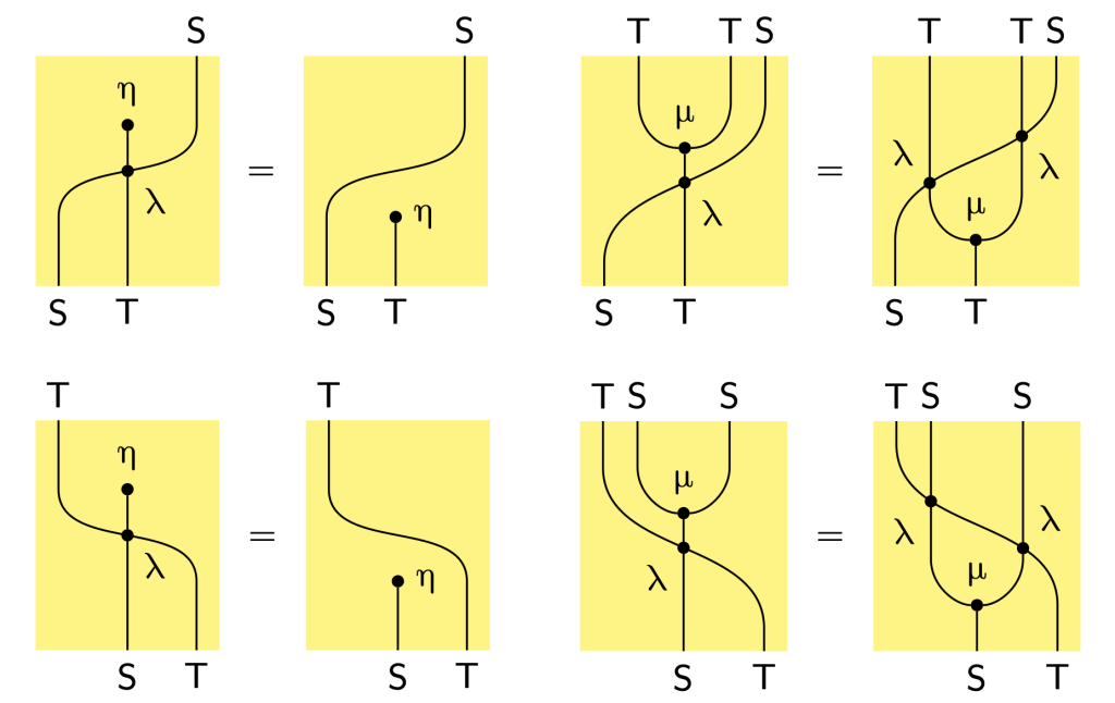
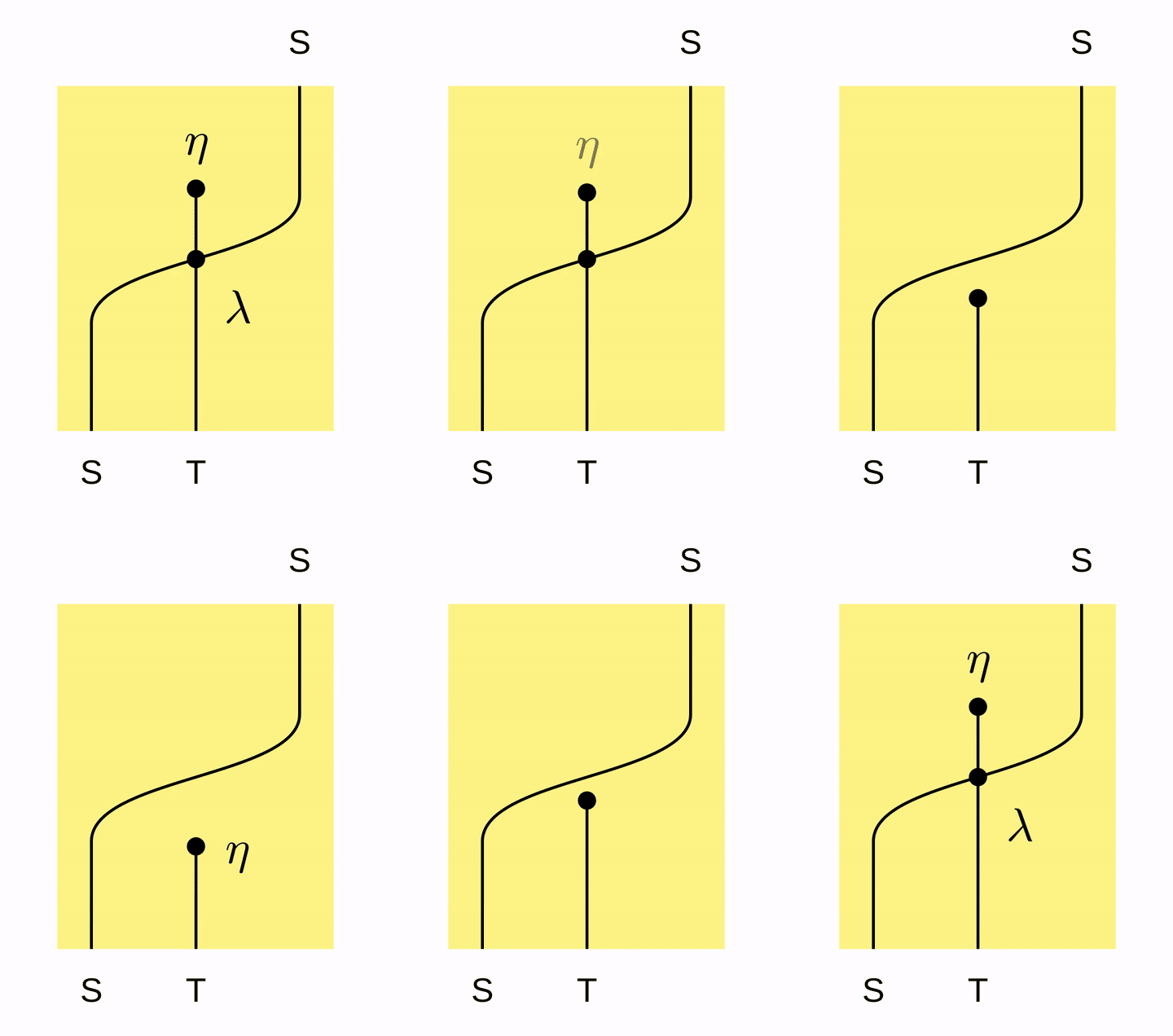
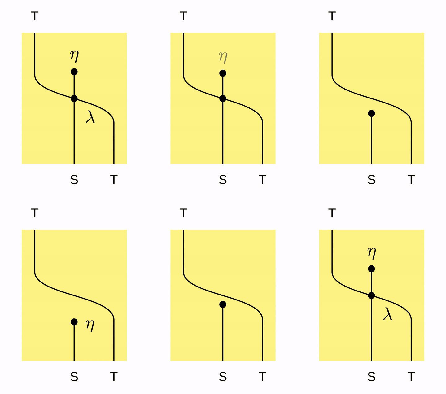
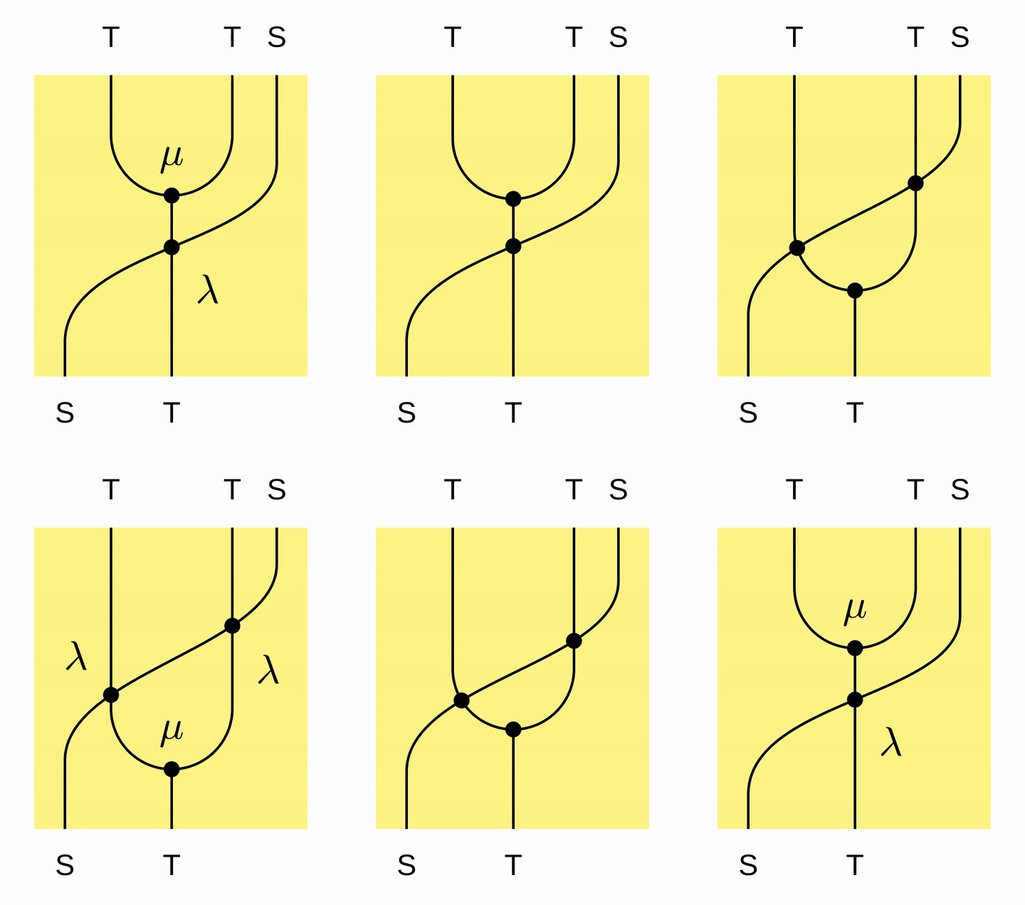
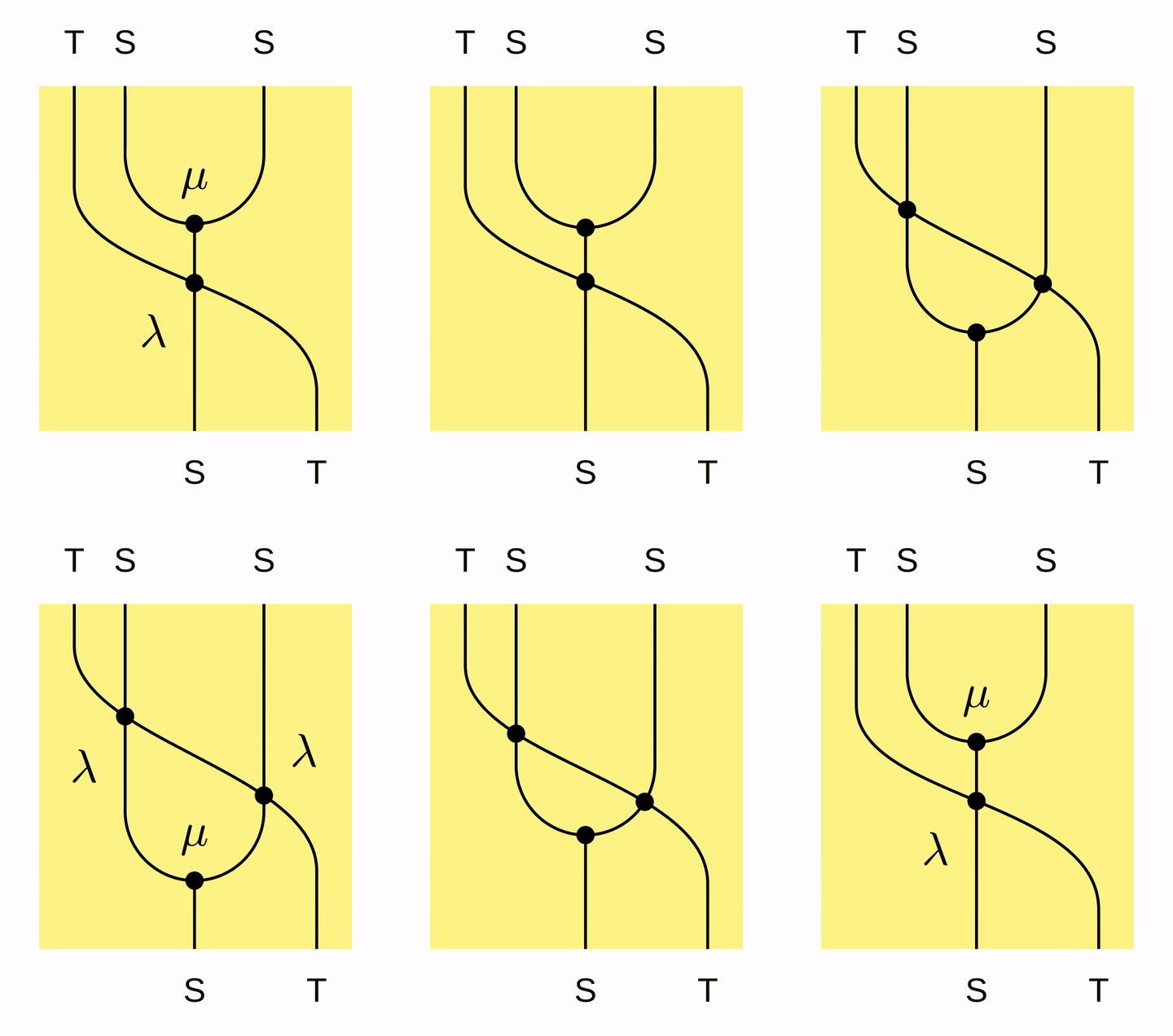
A commutative monad is a monoid in the category of lax symmetric monoidal endofunctors

We have seen the standard result that monad on a category $\mathcal{C}$ is a monoid in the endofunctor category

([\mathcal{C},\mathcal{C}],\otimes, \mathsf{Id})

We also discussed a similar result that a strong monad is a monoid in the category of strong endofunctors. That result allowed us to very directly read off what a distributive law of strong monads should be. The aim of this post is to continue this pattern for commutative monads, with the aim of recovering the definition of distributive law of commutative monads. This will turn out to take a bit more effort.

What we are not going to do

The first thing we should note is that we are not heading towards a result of the form:

A commutative monad is a commutative monoid in…

Unfortunately the term commutative monad hints at the wrong intuition in this regard.

Commutative Monads are Monoidal Monads

Now we have avoided a potential banana skin, onto the main story.

For a strong monad

(\mathbb{T} : \mathcal{C} \rightarrow \mathcal{C}, \eta, \mu, \mathsf{st} : X \otimes \mathbb{T}(Y) \rightarrow \mathbb{T}(X \otimes Y))

on a symmetric monoidal category

(\mathcal{C}, \otimes, I)

if the monad is commutative, the induced double strength

\mathsf{dst} : \mathbb{T}(X) \otimes \mathbb{T}(Y) \rightarrow \mathbb{T}(X \otimes Y)

gives our monad a symmetric monoidal structure. That is, $\mathbb{T}$ is a lax symmetric monoidal functor, and the unit and multiplication are monoidal natural transformations. In fact, we can also go in the other direction, given a symmetric monoidal monad with coherence map

\varphi : \mathbb{T}(X) \otimes \mathbb{T}(X) \rightarrow \mathbb{T}(X \otimes Y)

we can recover a corresponding left and right strength as the composites:

\varphi \cdot (\mathsf{id} \otimes \eta) : \mathbb{T}(X) \otimes Y \rightarrow \mathbb{T}(X \otimes Y)\quad\text{and}\quad \varphi \cdot (\eta \otimes \mathsf{id}) : X \otimes \mathbb{T}(Y) \rightarrow \mathbb{T}(X \otimes Y)

and we can travel back and forth between these two points of view. That is, a commutative monad is the same thing as a symmetric monoidal monad. Rephrasing again, for a symmetric monoidal category:

A commutative monad is a monoid in the category of lax symmetric monoidal endofunctors.

Distributive Laws of Commutative Monads

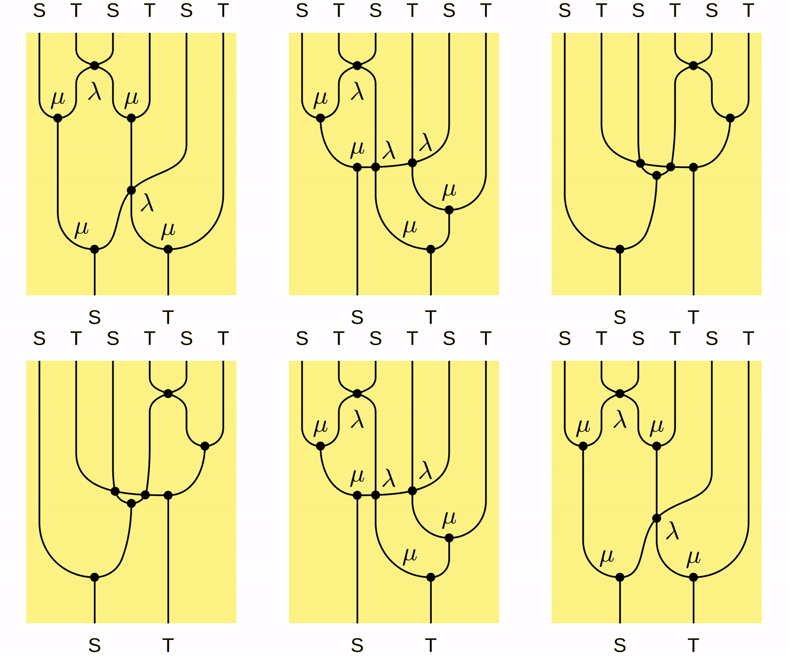
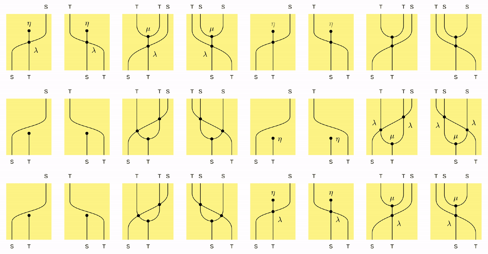
With the above observation in mind, a distributive law of commutative monads should be an ordinary distributive law

\lambda : \mathbb{S} \otimes \mathbb{T} \Rightarrow \mathbb{T} \otimes \mathbb{S}

which is also a monoidal natural transformation. Concretely, this means

\mathbb{T} \mathsf{dst}^{\mathbb{S}} \cdot \mathsf{dst}^{\mathbb{T}} \cdot \lambda \otimes \lambda = \lambda \cdot \mathbb{S} \mathsf{dst}^{\mathbb{T}} \cdot \mathsf{dst}^{\mathbb{S}}

The definition of a distributive law of commutative monads appearing in the literature in independent work of Wolff and Jacobs is a distributive law of strong monads, satisfying the additional equation

\lambda \cdot \mathbb{S}\mathsf{st’}^{\mathbb{T}} \cdot \mathsf{st}^{\mathbb{S}} = \mathbb{T}\mathsf{st}^{\mathbb{S} \cdot \mathsf{st’}^{\mathbb{T}}}

which involves a slightly odd combination of left and right strengths. Its not immediately obvious how the equation we have derived relates to the Wolff Jacobs conditions. So we have work to do.

A reasonably straightforward direct calculation shows that our equation implies the Wolff Jacobs conditions. Trying to proceed directly in the other direction proves significantly more painful.

Instead, we proceed indirectly. It is not too hard to show that composing two commutative monads using a distributive law of commutative monads result in a commutative monad. This is not a big shock, as it is their very purpose. By an observation of Beck, we can recover a distributive law from its composite monad by suitably precomposing the composite multiplication with the units of the component monads. We then note

The component monads are commutative by assumption, and so their units are monoidal.
The composite monad is commutative as a result of the Wolff Jacobs conditions, and so its multiplication is monoidal.
Becks composite recovering the distributive law combines only monoidal components.

Therefore, a distributive law satisfying the Wolff Jacobs conditions is a monoidal natural transformation.

Summing up, a distributive law of commutative monads is an ordinary distributive law that equivalently either:

Satisfies the Wolff Jacobs equations directly involving strength, or
Is a monoidal natural transformation

Summary

Monads and their distributive laws are 2-categorical phenomena, and so the correct definition of distributive law should be inevitable.

In a previous post we saw that the notion of distributive of strong monads appearing in the literature drops out directly from the abstract framework. In this post we moved on to look at the accepted notion of distributive law of commutative monads. The situation was more subtle, but it is reassuring that after a bit of massaging, instantiating the abstract definition yields the same construction.

Distributive laws of commutative monads appear in:

Wolff “Commutative Distributive Laws”
Jacobs “Semantics of weakening and contraction”

Distributive Laws and Tensor Products of Enriched Categories

Distributive laws are a fundamental concept in monad theory. They allow us to form well-behaved composite monads, lift monads to Kleisli and Eilenberg-Moore categories, and play key roles in various computer science applications.

As with any worthwhile mathematical object, it is useful to have multiple perspectives to clarify the underlying idea. This post aims to show how we might rediscover the notion of distributive from an enriched category theory point of view.

Monads and Enrichment

For a monoidal category $(\mathcal{V}, \otimes, I)$ , we can:

Define $\mathcal{V}$ -enriched categories, more concisely referred to as $\mathcal{V}$ -categories.
Define $\mathcal{V}$ -functors between $\mathcal{V}$ -categories.
If $\mathcal{V}$ is a symmetric monoidal category, we can define a tensor product of $\mathcal{V}$ -categories $\mathcal{C}$ and $\mathcal{D}$ , denoted $\mathcal{C} \otimes \mathcal{D}$ , generalising product categories from ordinary category theory.

We considered monads from an enriched point of view in a previous post. For our current discussion, we slightly vary the emphasis, and consider monads on a fixed category $\mathcal{C}$ (or more generally object in a 2-category). We enrich over the endofunctor category $[\mathcal{C},\mathcal{C}]$ with functor composition as the monoidal structure.

In this setting:

A monad $(\mathbb{T} : \mathcal{C} \rightarrow \mathcal{C}, \eta, \mu)$ is a one object $[\mathcal{C}, \mathcal{C}]$ -category, which we shall denote $\mathbb{T}$ . The unit and multiplication of the monad encode the identities and composition of the category, and the monad axioms ensure they behave as expected.
A monad map is the same things as a $[\mathcal{C}, \mathcal{C}]$ -functor, encoding the functor action on the hom object, with the monad map axioms enforcing preservation of identities and commuting with composition.
The monoidal category $([\mathcal{C}, \mathcal{C}], \otimes, \mathsf{Id})$ is clearly not symmetric. How do we get an analog of the tensor product of enriched categories?

The tensor product of $\mathcal{V}$ categories has objects pairs of objects from the components categories, and hom objects given by the tensor product of the component homs:

(\mathcal{C} \otimes \mathcal{D})((c_1, d_1), (c_2, d_2)) = \mathcal{C}(c_1,c_2) \otimes \mathcal{D}(d_1,d_2)

In order to define the composition maps

(\mathcal{C} \otimes \mathcal{D})((c_2,d_2),(c_3, d_3)) \otimes (\mathcal{C} \otimes \mathcal{D})((c_1,d_1),(c_2,d_2)) \rightarrow (\mathcal{C} \otimes \mathcal{D})((c_1,d_1),(c_3,d_3))

from the composition maps in the component categories, we need the assumption $\mathcal{V}$ is symmetric to allow us to wire things up in the right order.

Now if we consider our case of interest, monads

(\mathbb{S}, \eta, \mu) \quad\text{and}\quad(\mathbb{T},\eta,\mu)

viewed as one-object $[\mathcal{C}, \mathcal{C}]$ -categories, if we could form the tensor product of these categories,

\mathbb{T} \otimes \mathbb{S}

it would have a single hom object

\mathbb{T} \circ \mathbb{S}

As we have no symmetry, we need to figure out how to form a composition map

\mathbb{T} \circ \mathbb{S} \circ \mathbb{T} \circ \mathbb{S} \Rightarrow \mathbb{T} \circ \mathbb{S}

using the composition maps (monad multiplications) in the component categories. Following the standard tensor product construction, we need a natural transformation

\lambda : \mathbb{S} \circ \mathbb{T} \Rightarrow \mathbb{T} \circ \mathbb{S}

to swap the middle two components of the domain as follows:

\mathbb{T} \circ \mathbb{S} \circ \mathbb{T} \circ \mathbb{S} \xRightarrow{\mathbb{T} \circ \lambda \circ \mathbb{S}} \mathbb{T} \circ \mathbb{T} \circ \mathbb{S} \circ \mathbb{S}

Not any old natural transformation will do, in order to prove the resulting composition map is unital and associative, we will need some equational axioms. In fact, what we need is a distributive law!

Summary

This post stems from a simple line of reasoning:

Monads are special enriched categories
There are standard ways of composing monads and composing enriched categories, are these also related?

I would be very interested to understand if there is a well-known construction on enriched categories of which the perspective on distributive laws above is a special case?

A Strong Monad is Monoid in the Category of Strong Endofunctors

We encountered the notion of strength when we introduced strong monads. Strength has turned out to be an important idea, for example in discussion of commutative monads which underpin a lot of monad theory.

As strength is so important, we are going to back up, and examine it in a bit more detail, eventually arriving at a concise definition of strong monad.

Our ulterior motive is to set up some background on strong natural transformations so we can learn more about commutative, affine, relevant and cartesian monads in future posts.

Strong functors

Recall, a strength for an endofunctor

F : \mathcal{C} \rightarrow \mathcal{C}

on a monoidal category is a natural transformation

\mathsf{st} : X \otimes F(Y) \Rightarrow F (X \otimes Y)

compatible with the monoidal left unitor and associator, in that

F \lambda \cdot \mathsf{st} = \lambda

and

F \alpha \cdot \mathsf{st} = \mathsf{st} \cdot \mathsf{id} \otimes \mathsf{st} \cdot \alpha

A strong functor is a pair

(F, \mathsf{st} : X \otimes F(Y) \Rightarrow F(X \otimes Y))

consisting of an endofunctor and a choice of strength.

Strong natural transformations

We now introduce the key notion of this post. A strong natural transformation

\varphi : (F,\mathsf{st}) \rightarrow (G,\mathsf{st})

is an ordinary natural transformation

\varphi : F \Rightarrow G

which commutes with strengths. That is:

\mathsf{st} \cdot \mathsf{id} \otimes \varphi = \varphi \cdot \mathsf{st}

We will overload the symbol $\mathsf{st}$ for any strength to avoid a proliferation of symbols.

Categorical Structure

For a monoidal category $\mathcal{C}$ there is a category $\mathsf{Strong(\mathcal{C})}$ with:

Objects: Strong endofunctors on $\mathcal{C}$
Morphisms: Strong natural transformations, with composition and identities as for ordinary natural transformations.

Checking the required closure properties of strong natural transformations is a routine exercise.

Monoidal Structure

For a monoidal category $\mathcal{C}$ , there is a strict monoidal structure on $\mathsf{Strong}(\mathcal{C})$ with unit

(\mathsf{Id}_{\mathcal{C}}, \mathsf{id})

The tensor product on objects is:

(G,\mathsf{st}) \circ (F, \mathsf{st}) = (G \circ F, X \otimes GF(Y) \xrightarrow{\mathsf{st}}G(X \otimes F(Y)) \xrightarrow{G \mathsf{st}} GF(X \otimes Y))

For morphisms

\varphi : (F_1, \mathsf{st}) \Rightarrow (F_2, \mathsf{st}) \quad\text{and}\quad \gamma : (G_1, \mathsf{st}) \Rightarrow (G_2, \mathsf{st})

their tensor product is the usual composition of natural transformations

\gamma \circ \varphi : G_1 \circ F_1 \Rightarrow G_2 \circ F_2

Verifying the monoidal structure is routine, if fiddly, exercise in applying the definitions.

Strong Monads

When we previously discussed strong monads, the definition was only sketched, with detailed deferred to other sources. We are now in a position to give a precise definition of what a strong monad is

A strong monad is a monoid in the category of strong endofunctors.

This is easy to remember, as it is a small variation on the internets favourite meme about monads:

A monad is a monoid in the category of endofunctors.

We just sprinkle the term strong over the slogan for monads, and we get the corresponding slogan for strong monads.

It is not hard to see that there is a strict monoidal forgetful functor to the ordinary category of endofunctors

\mathsf{Strong}(\mathcal{C}) \rightarrow [\mathcal{C}, \mathcal{C}]

so every strong monad is an ordinary monad, along with some additional strength data.

Unpacking the Definition

If we unpack the concise definition above, a strong monad is:

A strong endofunctor $(\mathbb{T} : \mathcal{C} \rightarrow \mathcal{C}, \mathsf{st})$
A unit strong natural transformation $(\mathsf{Id}, \mathsf{id}) \Rightarrow (\mathbb{T}, \mathsf{st})$
A multiplication strong natural transformation $(\mathbb{T},\mathsf{st}) \circ (\mathbb{T}, \mathsf{st}) \Rightarrow (\mathbb{T}, \mathsf{st})$

Such that the usual unit and multiplication axioms hold.

Applying the Definition

To show that this is not just an exercise in meme generation, we can apply the definition above to deduce what a distributive law of strong monad $(\mathbb{T}, \mathsf{st})$ over strong monad $(\mathbb{S}, \mathsf{st})$ should be. We require a strong natural transformation:

\lambda : (\mathbb{T}, \mathsf{st}) \circ (\mathbb{S}, \mathsf{st}) \Rightarrow (\mathbb{S}, \mathsf{st}) \circ (\mathbb{T}, \mathsf{st})

satisfying formally identical equations to those of an ordinary distributive law. Unpacking this, $\lambda$ must be an ordinary distributive law, also satisfying:

\mathbb{S}(\mathsf{st}) \cdot \mathsf{st} \cdot 1 \otimes \lambda = \lambda \cdot \mathbb{T}(\mathsf{st}) \cdot \mathsf{st}

This yields the same definition given in Jacobs “Semantics of Weakening and Contraction” for example.

Summary

By identifying the correct mathematical structure, we have arrived at a concise definition of strong monad paralleling one of the familiar definitions for monads.

Inquisitive readers may wonder if any of the other definitions transfer over cleanly. For example, can we define a strong monad as a monad in a different 2-category? The answer is not yet (except in a rather degenerate way)! As with most things, there is a more general definition of strength, which amongst other things allows us to move away from the restriction to endofunctors that has been conspicuous in this post. Our current level of generality will be sufficient for some forthcoming posts. We may return to this topic on a later occasion. Details can be found on the NLab for example.

Distributive Laws and General Equations

We have seen we can distribute any monad $\mathbb{T}$ presented by linear equations over a commutative monad $\mathbb{S}$ . There is a balance between the assumptions on these two monads that yields a distributive law, but it is not the only choice. This time we look at strengthening our assumptions about the monad $\mathbb{S}$ so that we can weaken the restriction to presentations by linear equations on monad $\mathbb{T}$ and still have a distributive law.

The plan is quite simple. The previous results hinged on closure properties of multilinear extensions. Our approach is to consider classes of monads where we get stronger closure properties of multilinear extensions, so we continue to use uniqueness of multilinear extensions as our proof principle.

Special Classes of Monads

Throughout this post, $\mathbb{S}$ will denote a commutative monad on a category with finite products.

Recall that $\mathbb{S}$ is:

Affine if $\langle \mathbb{S} \pi_1, \mathbb{S} \pi_2 \rangle \cdot \mathsf{dst} = \mathsf{id}_{\mathbb{S}(X) \times \mathbb{S}(Y)}$ .
Relevant if $\mathsf{dst} \cdot \langle \mathbb{S}\pi_1, \mathbb{S}\pi_2 \rangle = \mathsf{id}_{\mathbb{S}(X \times Y)}$
Cartesian if it is both affine and linear.

Frustratingly, there are several unrelated notions of Cartesian monad used in the literature, so some caution with this terminology is required.

Multilinear Extensions for Affine Monads

We begin by investigating a special case of when we can delete inputs and still get multilinear extensions.

Assume $\mathbb{S}$ is an affine monad, and

\hat{h} : \mathbb{S}(X) \rightarrow \mathbb{S}(X)

is the multilinear extension of

h : X \rightarrow X

then the composite

\hat{h} \cdot \pi_1 : \mathbb{S}(X) \times \mathbb{S}(X) \rightarrow \mathbb{S}(X)

is the multilinear extension of

h \cdot \pi_1 : X \times X \rightarrow X

Intuitively, we can drop the second input and still get a multilinear extension.

To confirm multilinearity,

\hat{h} \cdot \pi_1 \cdot \mu \times \mu = \hat{h} \cdot \mu \cdot \pi_1 = \mu \cdot \mathbb{S}(\hat{h}) \cdot \pi_1

= \mu \cdot \pi_1 \mathbb{S}(\hat{h}) \cdot \pi_1 \cdot \langle \mathbb{S}\pi_1, \mathbb{S}\pi_2 \rangle \cdot \mathsf{dst} = \mu \cdot \mathbb{S}(\hat{h}) \cdot \mathbb{S}\pi_1 \cdot \mathsf{dst}

where the second step uses the assumed multilinearity of $\hat{h}$ , and the third step uses the assumption $\mathbb{S}$ is affine.

Verifying the extension property is a routine application of naturality.

Generalising from this special case, multilinear extensions of affine monads are closed under deleting variables. Using the same argument as the previous post, affine monads preserve equations that delete but don’t duplicate variables. We will refer to such equations as strictly deleting, and use the term strictly deleting presentation in the obvious way.

Multilinear Extensions for Relevant Monads

We begin by looking at a special case of when we can duplicate inputs and still get a multilinear extension.

Assume $\mathbb{S}$ is a relevant monad, and

\hat{h} : \mathbb{S}(X) \times \mathbb{S}(X) \rightarrow \mathbb{S}(X)

is the multilinear extension of

h : X \times X \rightarrow X

then the composite

\hat{h} \cdot \Delta_{\mathbb{S}(X)} : \mathbb{S}(X) \rightarrow \mathbb{S}(X)

is the multilinear extension of

h \cdot \Delta_{X} : X \rightarrow X

(Here $\Delta$ is the usual diagonal or copying natural transformation.) Intuitively we can duplicate the input and still get a multilinear extension.

To confirm multilinearity,

\hat{h} \cdot \Delta \cdot \mu = \hat{h} \cdot \mu \times \mu \cdot \Delta = \mu \cdot \mathbb{S}(\hat{h}) \cdot \mathsf{dst} \cdot \Delta

= \mu \cdot \mathbb{S}(\hat{h}) \cdot \mathsf{dst} \cdot \langle \mathbb{S} \pi_1, \mathbb{S} \pi_2 \rangle \cdot \mathbb{S}(\Delta) = \mu \cdot \mathbb{S}(\hat{h}) \cdot \mathbb{S}(\Delta)

where the second step uses the assumed multilinearity, and the final step uses relevance of $\mathbb{S}$ .

Again, verifying the extension property is straightforward.

Generalising from this special case, multilinear extensions of relevant monads are closed under duplicating variables. Again, using the same argument as the previous post, relevant monads preserve equations that duplicate but don’t delete variables. We will refer to such equations as strictly duplicating, and use the term strictly duplicating presentation in the obvious way.

Consequences

Combining the proof principle of uniqueness of multilinear extensions with the additional closure properties above, we get a range of results. For a commutative monad $\mathbb{T}$ there is a distributive law:

\mathbb{T} \circ \mathbb{S} \Rightarrow \mathbb{S} \circ \mathbb{T}

$\mathbb{T}$ has a linear presentation.
$\mathbb{S}$ is affine and $\mathbb{T}$ has a strictly deleting presentation.
$\mathbb{S}$ is relevant and $\mathbb{T}$ has a strictly duplicating presentation.
$\mathbb{S}$ is Cartesian and $\mathbb{T}$ is any finitary monad.

Summary

The preservation theorems involving affine, relevant and Cartesian monads appear in the PhD thesis of Louis Parlant, although the proof strategy was somewhat different. Continuing Manes emphasis on multilinear maps provides a uniform perspective on all the different results.

Linearity, Laws and Liftings

We have seen that we can extend algebraic operations to powersets, and these extensions preserve linear equations. This allowed us to lift the powerset monad to the Eilenberg-Moore category of a monad presented by linear equations. Equivalently, this gives us sufficient conditions for a monad to distribute over the powerset monad.

Now we have some general results about multilinear extensions, we are finally at the point when we can:

Generalise the monad lifting and distributive law results we have seen so far beyond the powerset monad.
Identify what is special about linear equations that makes these constructions work.

The payoff will be theorems yielding lifted monads and distributive laws.

Closure Properties of Multilinear Morphism

We will work in a symmetric monoidal category, which we assume to be strict to keep discussions simple.

A first unsurprising result is that multilinear maps are closed under permutations of their arguments. Formally, if

\hat{f} : \mathbb{S}(X) \otimes \ldots \otimes \mathbb{S}(X) \rightarrow \mathbb{S}(X)

is the multilinear extension of

f : X \otimes \ldots \otimes X \rightarrow X

and

s_X : X \otimes \ldots \otimes X \rightarrow X \otimes \ldots \otimes X

is a natural transformation describing a permutation built using the symmetry natural transformation, then

\hat{f} \cdot s_{\mathbb{S}(X)} : \mathbb{S}(X) \otimes \ldots \otimes \mathbb{S}(X) \rightarrow \mathbb{S}(X)

is the multilinear extension of

f \cdot s_{X} : X \otimes \dots \otimes X \rightarrow X

The proof is a completely routine.

An important, and only slightly less obvious closure property is that multilinear extensions are closed under composition. For example, if

\hat{f}, \hat{g}, \hat{h} : \mathbb{S}(X) \otimes \mathbb{S}(X) \rightarrow \mathbb{S}(X)

are the respective bilinear extensions of

f,g,h : X \otimes X \rightarrow X

then the composite

h \cdot (f \otimes g) : \mathbb{S}(X) \otimes \mathbb{S}(X) \otimes \mathbb{S}(X) \otimes \mathbb{S}(X) \rightarrow \mathbb{S}(X)

is the multilinear extension of

h \cdot (f \otimes g) : X \otimes X \otimes X \otimes X \rightarrow X

The proof is another routine diagram chase.

Preservation of Linear Equations

We now return to the setting of algebraic structures on sets. Consider a structure with binary operations:

f,g,h : X \times X \rightarrow X

satisfying the linear equation:

h(f(w,x),g(y,z)) = h(g(y,z),f(w,x))

We can rephrase this in terms of composite morphisms as:

h \cdot (f \times g) = h \cdot (g \times f) \cdot s_X

where $s$ is the natural transformation that orders the arguments on the righthand side correctly.

Using the closure properties of multilinear extensions, the composites:

\hat{h} \cdot (\hat{f} \times \hat{g}) \quad\text{and}\quad \hat{h} \cdot (\hat{g} \times \hat{f}) \cdot s_{\mathbb{T}(X)}

are multilinear extensions of the left and right hand side of the previous equation. By the uniqueness of multilinear extensions:

\hat{h} \cdot (\hat{f} \times \hat{g}) = \hat{h} \cdot (\hat{g} \times \hat{f}) \cdot s_{\mathbb{T}(X)}

and so the equation lifts from $X$ to multilinear extensions of the operations on $\mathbb{S}(X)$ .

Note this argument would not work for equations that are not linear. The whole argument hinges on the proof principle that multilinear extensions are unique, but we have no closure property of multilinear extensions that allows us to drop or duplicate arguments. We will return to this topic in the next post.

We can generalise the above argument to an arbitrary linear equation, and so all such equations are preserved when extending operations to their multilinear extensions on $\mathbb{S}(X)$ .

Consequences

If monad $\mathbb{S}$ is commutative and monad $\mathbb{T}$ has a presentation only requiring linear equations:

The monad $\mathbb{S}$ lifts to the category $\mathsf{Set}^{\mathbb{T}}$ .
There is a distributive law of type $\mathbb{T} \circ \mathbb{S} \Rightarrow \mathbb{S} \circ \mathbb{T}$ .

Example: The multiset monad is both commutative and presented by linear equations. Therefore:

For any commutative monad $\mathbb{S}$ there is a distributive law of type $\mathbb{M} \circ \mathbb{S} \Rightarrow \mathbb{S} \circ \mathbb{M}$ .
For any monad $\mathbb{T}$ with a presentation by linear equations, there is a distributive law of type $\mathbb{T} \circ \mathbb{M} \Rightarrow \mathbb{M} \circ \mathbb{T}$ .

In particular, the multiset monad distributes over itself.

Summary

These results appear in Manes and Mulry “Monad Compositions I”, and many distributive laws arise in this way. These results are well-known, but the restriction linear equations is frustrating. In the next post, we will look at more recent results making a slightly different trade-off to circumvent the restriction to linear equations.

Distributing over the powerset

We saw in the previous post that we can lift the powerset monad to a monad on any category of algebras defined by linear equations. In this short post, we shall tidy some loose ends, leading to another perspective on what we have done.

Eilenberg-Moore Algebras

As we have discussed previously, every finitary monad

(\mathbb{T} : \mathsf{Set} \rightarrow \mathsf{Set}, \eta, \mu)

arises from the free / forgetful adjunction of an equationally defined category of algebras:

\mathsf{Alg}(\Sigma,E)

Furthermore, the Eilenberg-Moore category $\mathsf{Set}^{\mathbb{T}}$ is equivalent to $\mathsf{Alg}(\Sigma,E)$ .

Putting these two facts together, if $\mathbb{T}$ has a presentation only involving linear equations, the previous post shows that the powerset monad lifts to a monad:

(\hat{\mathbb{P}} : \mathsf{Set}^{\mathbb{T}} \rightarrow \mathsf{Set}^{\mathbb{T}}, \hat{\eta}, \hat{\mu})

We have encountered liftings to Eilenberg-Moore categories before. In that case, we were interested in lifting functors to Eilenberg-Moore categories. In this case, we are interested in lifting entire monads.

For monads:

(\mathbb{S}, \eta, \mu)\quad\text{and}\quad(\mathbb{T}, \eta, \mu)

there is a bijection between:

Liftings of the monad $\mathbb{S}$ to $\mathsf{Set}^{\mathbb{T}}$ .
Distributive laws of type $\mathbb{T} \circ \mathbb{S} \Rightarrow \mathbb{S} \circ \mathbb{T}$ .

This is a topic worthy of further discussion, which we will return to in a later post.

Combining this bijection with the previous observation, if the monad $\mathbb{T}$ has a presentation by linear equations, there is a distributive law:

\mathbb{T} \circ \mathbb{P} \Rightarrow \mathbb{P} \circ \mathbb{T}

Summing Up

Using some standard facts, and Gautam’s results about extending algebraic structure to powersets, we have found sufficient conditions for the existence of a distributive law of $\mathbb{T}$ over the powerset monad $\mathbb{P}$ .

Our next steps is to clarify at a higher level of abstraction what is going on, so we can move beyond the powerset to more general monads.

Distributive Laws are Monads

Early on we claimed, with no explanation, that distributive laws are monads. As the title of this post suggests, we are now in a place to explain the details of what this rather intriguing statement means. This will require our previous experience of monads in a 2-category, and distributive laws. In particular, the ability to define monads within arbitrary 2-categories gives us an awful lot of additional expressive freedom. Our first step will be to introduce a 2-category suitable for formalising relationships between monads.

A 2-category of Monads

The 2-category that we will be interested in has monads as 0-cells, Eilenberg-Moore laws as 1-cells, and compatible natural transformations as 2-cells. We now spell out the details.

For an arbitrary 2-category $\mathbf{K}$ , there is a 2-category $\mathbf{Mnd}(\mathbf{K})$ with:

0-cells: Tuples $(\mathcal{C}, \mathbb{T}, \eta, \mu)$ consisting of a 0-cell $\mathcal{C}$ , such that $(\mathbb{T},\eta,\mu)$ is a monad on $\mathcal{C}$ in $\mathbf{K}$ .
1-cells: A 2-cell $(\mathcal{C}, \mathbb{S}, \eta^{\mathbb{S}}, \mu^{\mathbb{S}}) \rightarrow (\mathcal{D}, \mathbb{T}, \eta^{\mathbb{T}}, \mu^{\mathbb{T}})$ is a pair $(U,\varphi)$ consisting of a 1-cell $U : \mathcal{C} \rightarrow \mathcal{D}$ , and a 2-cell $\varphi : \mathbb{T} \circ U \Rightarrow U \circ \mathbb{S}$ , such that $\varphi$ is an Eilenberg-Moore law.
2-cells: A 2-cell $(U,\varphi) \Rightarrow (U',\varphi')$ is a 2-cell $\sigma : U \Rightarrow U'$ such that $\varphi' \cdot (\mathbb{T} \circ \sigma) = (\sigma \circ \mathbb{S}) \cdot \varphi$ .

Horizontal composition is given by

$(V,\psi : \mathbb{T} \circ V \Rightarrow V \circ \mathbb{S}) \circ (U,\varphi : \mathbb{S} \circ U \Rightarrow U \circ \mathbb{R}) = (V \circ U, (V \circ \varphi) \cdot (\psi \circ V))$

with

$\mathsf{Id}_{(\mathcal{C},\mathbb{T},\eta,\mu)} = (\mathsf{Id}_{\mathcal{C}}, \mathsf{id}_{\mathbb{T}})$

The vertical composition and identities for 2-cells in $\mathbf{Mnd}(\mathbf{K})$ are inherited from $\mathbf{K}$ .

Monads in the 2-category of Monads

We now consider what a monad in $\mathbf{Mnd}(\mathbf{K})$ boils down to. As we will be working a 2-category constructed from another 2-category, and with 3 different monads, we will be fussy in spelling out the details carefully.

A monad in $\mathbf{Mnd}(\mathbf{K})$ consists of four pieces of data:

A 0-cell in $\mathbf{Mnd}(\mathbf{K})$ . That is, some monad $(\mathcal{C}, \mathbb{S}, \eta^{\mathbb{S}}, \mu^{\mathsf{S}})$ in $\mathbf{K}$ .
A 1-cell in $\mathbf{Mnd}(\mathbf{K})$ of type $(\mathcal{C}, \mathbb{S}, \eta^{\mathbb{S}}, \mu^{\mathsf{S}}) \rightarrow (\mathcal{C}, \mathbb{S}, \eta^{\mathbb{S}}, \mu^{\mathsf{S}})$ . That is, a 1-cell $\mathbb{T} : \mathcal{C} \rightarrow \mathcal{C}$ in $\mathbf{K}$ , and an Eilenberg-Moore law $\lambda : \mathbb{S} \circ \mathbb{T} \Rightarrow \mathbb{T} \circ \mathbb{S}$ .
A unit 2-cell of type $\mathsf{Id}_{(\mathcal{C}, \mathbb{S}, \eta^{\mathbb{S}}, \mu^{\mathsf{S}})} \Rightarrow (\mathbb{T}, \lambda)$ in $\mathbf{Mnd}(\mathbf{K})$ . That is, a 2-cell $\eta^{\mathbb{T}} : \mathsf{Id}_{\mathcal{C}} \Rightarrow \mathbb{T}$ in $\mathbf{K}$ such that $\lambda \cdot (\mathbb{S} \circ \eta^{\mathbb{T}}) = \eta^{\mathbb{T}} \circ \mathbb{S}$ .
A multiplication 2-cell of type $(\mathbb{T}, \lambda) \circ (\mathbb{T}, \lambda) \Rightarrow (\mathbb{T}, \lambda)$ in $\mathbf{Mnd}(\mathbf{K})$ . That is, a 2-cell $\mu^{\mathbb{T}} : \mathbb{T} \circ \mathbb{T} \Rightarrow \mathbb{T}$ in $\mathbf{K}$ such that $\lambda \cdot (\mathbf{S} \circ \mu^{\mathbb{T}}) = \mu^{\mathbb{T}} \cdot (\mathbb{T} \circ \lambda) \cdot (\lambda \circ \mathbb{T})$ .

The unit and associativity axioms for a monad in $\mathbf{Mnd}(\mathbf{K})$ are equivalent to requiring that $(\mathbb{T}, \eta^{\mathbb{T}}, \mu^{\mathbb{T}})$ satisfies those axioms for a monad on $\mathcal{C}$ in $\mathbf{K}$ . Finally, the two equations satisfied by the unit and multiplication as 2-cells in $\mathbf{Mnd}(\mathbf{K})$ are equivalent to requiring that $\lambda$ is a Kleisli-law. As we noted previously, being a distributive law is equivalent to simultaneously being an Eilenberg-Moore law and a Kleisli law. Therefore, a monad in $\mathbf{Mnd}(\mathbf{K})$ is equivalent to the following data:

A 0-cell $\mathcal{C}$ in $\mathbf{K}$ .
A pair of monads $(\mathbf{S}, \eta^{\mathbb{S}}, \mu^{\mathbb{S}})$ and $(\mathbb{T}, \eta^{\mathbb{T}}, \mu^{\mathbb{T}})$ on $\mathcal{C}$ in $\mathbf{K}$ .
A distributive law $\mathbb{S} \circ \mathbb{T} \Rightarrow \mathbb{T} \circ \mathbb{S}$ in $\mathbf{K}$ .

Roughly speaking, up to being more careful to specify all the required data, a distributive law in $\mathbf{K}$ is the same thing as a monad in $\mathsf{Mnd}(\mathbf{K})$ .

Example: For the “ordinary” monads discussed in the previous post, a distributive law is a monad in $\mathbf{Mnd}(\mathbf{Cat})$ .

If we iterate the monad 2-category construction, a distributive law in $\mathbf{K}$ is the same thing as a 0-cell in $\mathbf{Mnd}(\mathbf{Mnd}(\mathbf{K}))$ .

Conclusion

This relatively short post has unravelled an observation of Street, to show how a distributive law can be seen as a monad in a suitable 2-category. This both served as an illustration of the power of the notion of monad in a 2-category, and provided an excuse to introduce the 2-category $\mathsf{Mnd}(\mathbf{K})$ . This 2-category is important more broadly in the theory of monads and distributive laws. In particular, by using the different dualities that apply in a 2-category, which we encountered when discussing comonads, we can incorporate comonads and Kleisli laws in the same setting. By iterating these constructions, we can consider different flavours of distributive laws such as monad-comonad or comonad-monad distributive laws. Hopefully we will get the chance to return to these topics later.

Further reading: The constructions outlined in this post were introduced in Street’s “Formal Theory of Monads”, along with vastly more important ideas than we have had chance to discuss. The 2-category $\mathsf{Mnd}(\mathbf{K})$ is also discussed in a very readable way, with more motivation for computer scientists, in Power and Watanabe’s “Combining a Monad and a Comonad”, along with many other interesting developments.

Composition and Distributive Laws

A common theme in many scientific disciplines is the desire to build up complicated objects out of simpler parts. This compositional perspective allows us to work in a modular fashion, rather than addressing each new problem as a monolith that must be investigated from scratch.

With this in mind, given two monads $\mathbb{T}, \mathbb{S}$ , it would be very convenient if the composite endofunctor $\mathbb{T} \circ \mathbb{S}$ was also a monad in some canonical way. Unfortunately, this is not always the case. Although this is initially disappointing, the study of when such composites are monads is a rich and interesting subject.

Composing Endofunctors

We begin with some simple concrete examples, to get a sense of the various possibilities when we try to compose two monads as endofunctors. We will say that an endofunctor $F$ can be given the structure of a monad, if there exists any $\eta : \mathsf{Id} \Rightarrow F$ and $\mu : F \circ F \Rightarrow F$ satisfying the unit and associativity axioms. We then note the following instructive examples:

Trivially, for any monad $\mathbb{S}$ , both the composites with the identity monad $\mathsf{Id} \circ \mathbb{S}$ and $\mathbb{S} \circ \mathsf{Id}$ carry the structure of a monad. As an equally trivial corollary of this observation, as there are endofunctors that carry multiple monad structures, this will also be a possibility for composite monads.
For any monad $\mathbb{S}$ , its post composition with the exception monad $\mathbb{S}(- + E)$ carries the structure of a monad.
The composition of the powerset monad with itself $\mathbb{P} \circ \mathbb{P}$ does not carry the structure of a monad. This was shown by Klin and Salamanca “Iterated Covariant Powerset is not a Monad” in 2018.

This is a pretty mixed picture. There are monads such that composition with their endofunctor on one or both sides results in a monad every time, and at the other extreme, some monads can’t even be composed with themselves.

Distributive Laws

Our aim now is to try and deduce some sufficient conditions under which monads compose. We will consider two monads $(\mathbb{S}, \eta^{\mathbb{S}}, \mu^{\mathbb{S}})$ and $(\mathbb{T},\eta^{\mathbb{T}}, \mu^{\mathbb{T}})$ on the same base category. Our notation is a bit fussier than normal, using superscripts on the unit and counit to make it clear which monad is intended.

We would like to find a monad structure on $\mathbb{T} \circ \mathbb{S}$ . There is an obvious choice for the unit:

$\eta^{\mathbb{T}} \circ \eta^{\mathbb{S}} : \mathsf{Id} \Rightarrow \mathbb{T} \circ \mathbb{S}$

If we trying composing the two multiplications together in the same way, we get:

$\mu^{\mathbb{T}} \circ \mu^{\mathbb{S}} : \mathbb{T} \circ \mathbb{T} \circ \mathbb{S} \circ \mathbb{S} \Rightarrow \mathbb{T} \circ \mathbb{S}$

We now see a problem, we have a natural transformation of type $\mathbb{T} \circ \mathbb{T} \circ \mathbb{S} \circ \mathbb{S} \Rightarrow \mathbb{T} \circ \mathbb{S}$ , not the type $\mathbb{T} \circ \mathbb{S} \circ \mathbb{T} \circ \mathbb{S} \Rightarrow \mathbb{T} \circ \mathbb{S}$ which we require. A natural attempt to address this problem would be to introduce some natural transformation $\lambda : \mathbb{S} \circ \mathbb{T} \Rightarrow \mathbb{T} \circ \mathbb{S}$ , and form the composite:

$(\mu^{\mathbb{T}} \circ \mu^{\mathbb{S}}) \cdot (\mathsf{Id}_{\mathbb{T}} \circ \lambda \circ \mathsf{Id}_{\mathbb{S}}) : \mathbb{T} \circ \mathbb{S} \circ \mathbb{T} \circ \mathbb{S} \Rightarrow \mathbb{T} \circ \mathbb{S}$

Of course, we can’t just use any old natural transformation $\lambda$ , it will need to satisfy some axioms in order for the resulting construction to be a monad. It is an interesting exercise to try and deduce these by attempting a proof, which I would highly recommend.

Sufficient conditions are two unit axioms:

$\lambda \cdot (\eta^{\mathbb{S}} \circ \mathbb{T}) = \mathbb{T} \circ \eta^{\mathbb{S}} \qquad \lambda \cdot (\mathbb{S} \circ \eta^{\mathbb{T}}) = \mathbb{S} \circ \eta^{\mathbb{T}}$

and two multiplication axioms:

$\lambda \cdot (\mathbb{T} \circ \mu^{\mathbb{S}}) = (\mathbb{T} \circ \mu^{\mathbb{S}}) \cdot (\lambda \circ \mathbb{S}) \cdot (\mathbb{S} \circ \lambda) \qquad \lambda \cdot (\mathbb{S} \circ \mu^{\mathbb{T}}) = (\mu^{\mathbb{T}} \circ \mathbb{S}) \cdot (\mathbb{T} \circ \lambda) \cdot (\lambda \circ \mathbb{T})$

A natural transformation $\lambda : \mathbb{S} \circ \mathbb{T} \Rightarrow \mathbb{T} \circ \mathbb{S}$ satisfying these four equations is known as a distributive law. This construction was first discovered by Jon Mock Beck, and they are sometimes referred to as Beck distributive laws for emphasis. Interestingly, the required axioms are exactly that $\lambda$ is both a Kleisli law and an Eilenberg-Moore law, which we encountered previously.

Of course, we haven’t actually demonstrated that such natural transformations can be found, so it’s time for some examples.

Example: For the free monoid (list) monad $\mathbb{L}$ , and the Abelian group monad $\mathbb{A}$ , there is a distributive law:

$\lambda : \mathbb{L} \circ \mathbb{A} \Rightarrow \mathbb{A} \circ \mathbb{L}$

We can think of the elements of $(\mathbb{L} \circ \mathbb{A})(X)$ as equivalence classes of products-of-sums, for example:

$(x_1 + x_2) \times (x_3 + x_4)$

If we apply the usual distributivity axiom for multiplication over addition, we get the term:

$x \times (y + z) = x \times y + x \times z$

our example term becomes a sum-of-products:

$x_1 \times x_3 + x_1 \times x_4 + x_2 \times x_3 + x_2 \times x_4$

which is an element of $(\mathbb{A} \circ \mathbb{L})(X)$ . This operation on terms is the idea behind the action of the distributive law, and also inspires the name distributive law. The resulting monad in the free ring monad.

Example: Again for the list and Abelian group monads, there is no distributive law composing in the opposite order, of the type:

$\mathbb{A} \circ \mathbb{L} \Rightarrow \mathbb{L} \circ \mathbb{A}$

This gives us an example of a pair of monads with a distributive law in one order, but not the other.

Example: Similarly to the ring monad example, there is a distributive law between the list and powerset monads:

$\mathbb{L} \circ \mathbb{P} \Rightarrow \mathbb{P} \circ \mathbb{L}$

The action of this distributive is:

$[X_1,\ldots,X_n] \mapsto \{ [x_1,\ldots,x_n] \mid x_i \in X_i \}$

As the powerset monad is the free complete join semilattice monad, and list is the free monoid monad, we can view the action of this distributive law algebraically as:

$\bigvee X_1 \otimes \ldots \bigvee X_n = \bigvee \{ x_1 \otimes \ldots \otimes x_n \mid x_i \in X_i \}$

Essentially, this distributive law comes from axioms of the form:

$x \otimes \bigvee Y = \bigvee \{ x \otimes y \in Y \} \qquad \bigvee X \otimes y = \{ x \otimes y \mid x \in X \}$

The algebras of the resulting monad are known as quantales.

Example: As a more computational example, consider the exception monad for any object $E$ , and and arbitrary monad $\mathbb{T}$ . There is a distributive law:

$\mathbb{T} + E \Rightarrow \mathbb{T}(- + E)$

Abstractly, this law has components:

$\mathbb{T}(X) + E \xrightarrow{[\mathbb{T}(\kappa_1), \eta^{\mathbb{T}} \circ \kappa_2]} \mathbb{T}(X + E)$

where $\kappa_1$ and $\kappa_2$ are the coproduct injections. For example, if we take monad $\mathbb{T}$ to be the list monad, the distributive law acts on the left component of the coproduct as:

$(0,[x_1,\ldots,x_n]) \mapsto [(0,x_1),\ldots,(0,x_n)]$

and on the right component:

$(1,e) \mapsto [(1,e)]$

The next example illustrates that distributive laws are only one aspect of the composition question for monads.

Example: As another negative result, there is no distributive law for the list monad over itself $\mathbb{L} \circ \mathbb{L} \Rightarrow \mathbb{L} \circ \mathbb{L}$ , but $\mathbb{L} \circ \mathbb{L}$ does carry the structure of a monad (as was pointed out by Bartek Klin). So the lack of a distributive law does not spell doom for finding any monad structure at all on the composite endofunctor.

Given the previous example, one might ask what are the advantages of knowing the composite monad $\mathbb{T} \circ \mathbb{S}$ arises via a distributive law? The key point is that we then get sensible relationships between the composite and its component parts. There are monad morphisms $\mathbb{S} \Rightarrow \mathbb{T} \circ \mathbb{S}$ and $\mathbb{T} \Rightarrow \mathbb{T} \circ \mathbb{S}$ . These in turn induce functors between the corresponding Kleisli and Eilenberg-Moore categories, as we have seen previously. Furthermore, $\mathbb{T}$ lifts to a monad on the Eilenberg-Moore category of $\mathbb{S}$ , and $\mathbb{S}$ lifts to a monad on the Kleisli category of $\mathbb{T}$ .

Conclusion

We have only touched on the topic of distributive laws in this post. Hopefully it’s fairly obvious to see that these ideas will generalise to the 2-categorical and bicategorical definitions of monads we recently discussed. There are results giving sufficient conditions, either for when a distributive laws does exist, or precluding that possibility. There is also a lot of open ground for new results in this area, showing that in some ways our understanding of monads is still rather naive.

For those interested in distributive laws, I would thoroughly recommend Jon Beck’s original 1969 paper, which is a very enjoyable read.

One final note of caution. Distributive laws are a notorious source of difficulty and errors in the literature. If you are working with them, or depending on the results of other, it is worth putting in extra effort to make sure you are on firm ground.

Example Laws and Liftings

We have now seen both Kleisli and Eilenberg-Moore laws, and their associated notions of lifted functor. Despite introducing the appropriate definitions, and sketching their key theoretical properties, we haven’t really seen any examples yet. That is the issue we now address.

A standard source of both Kleisli and Eilenberg-Moore laws are the monad morphisms $\sigma : \mathbb{S} \rightarrow \mathbb{T}$ . This can be seen as both

A Kleisli law of type $\mathsf{Id} \circ \mathbb{S} \Rightarrow \mathbb{T} \circ \mathsf{Id}$ .
An Eilenberg-Moore law of type $\mathbb{S} \circ \mathsf{Id} \Rightarrow \mathsf{Id} \circ \mathbb{T}$ .

Therefore, each monad morphism $\sigma$ induces both:

A functor $\underline{\mathsf{Id}} : \mathcal{C}_{\mathbb{S}} \rightarrow \mathcal{C}_{\mathbb{T}}$ such that $\underline{\mathsf{Id}} \circ F_{\mathbb{S}} = F_{\mathbb{T}}$ .
A functor $\overline{\mathsf{Id}}: \mathcal{C}^{\mathbb{T}} \rightarrow \mathcal{C}^{\mathbb{S}}$ such that $U_{\mathbb{S}} = U_{\mathbb{T}} \circ \overline{\mathsf{Id}}$ .

(Notice the difference in direction between the two).

Example: For every monad, the unit $\eta : \mathsf{Id} \Rightarrow \mathbb{T}$ is a monad morphism. For the identity monad there are obvious isomorphisms:

$\mathcal{C}_{\mathsf{Id}} \cong \mathcal{C} \cong \mathcal{C}^{\mathsf{Id}}$

Up to composition with these isomorphisms, the functor $\underline{\mathsf{Id}} : \mathcal{C}_{\mathsf{Id}} \rightarrow \mathcal{C}_{\mathbb{T}}$ is the usual Kleisli free functor, and the functor $\overline{\mathsf{Id}} : \mathcal{C}^{\mathbb{T}} \rightarrow \mathcal{C}^{\mathsf{Id}}$ is the usual Eilenberg-Moore forgetful functor.

As is a recurring theme, we should always consider what a new feature of monad theory means in terms of algebra.

Example: Consider two equational presentations over the same signature $(\Sigma, E), (\Sigma, E')$ such that $E \subseteq E'$ , with respective induced monads $\mathbb{S}, \mathbb{T}$ . Then for a set $A$ , every equivalence class of terms in $\mathbb{S}(A)$ is contained in an equivalence class of terms in $\mathbb{T}(A)$ , as the latter theory satisfies more equations. This induces a monad morphism:

$\mathbb{S} \Rightarrow \mathbb{T}$

The induced functor $\overline{\mathsf{Id}} : \mathsf{Set}^{\mathbb{T}} \rightarrow \mathsf{Set}^{\mathbb{S}}$ picks out the subcategory of $\mathbb{T}$ -algebras (which satisfy more equations), within the larger category of $\mathbb{S}$ -algebras. For example, every commutative monoid is a monoid.

As usual, we can consider the morphisms of $\mathsf{Set}_{\mathbb{S}}$ and $\mathsf{Set}_{\mathbb{T}}$ as families of equivalence classes of terms in the respective theories. From this point of view, every equivalence class in the weaker theory can be promoted to the enclosing one in the stronger theory. This is the behaviour of the induced functor $\underline{\mathsf{Id}} : \mathsf{Set}_{\mathbb{S}} \rightarrow \mathsf{Set}_{\mathbb{T}}$ . For example, the term $x + y$ in the theory of monoids will be mapped to an equivalence class including $y + x$ in the theory of commutative monoids.

We can also find examples beyond monad morphisms to show the greater generality is useful.

Example: For every monad, the multiplication $\mu : \mathbb{T} \circ \mathbb{T} \Rightarrow \mathbb{T}$ is both:

A Kleisli law of type $\mathbb{T} \circ \mathbb{T} \Rightarrow \mathsf{Id} \circ \mathbb{T}$ .
An Eilenberg-Moore law of type $\mathbb{T} \circ \mathbb{T} \Rightarrow \mathbb{T} \circ \mathsf{Id}$ .

Up to the isomorphisms discussed in the earlier example:

The induced functor $\underline{\mathbb{T}} : \mathcal{C}_{\mathbb{T}} \Rightarrow \mathcal{C}_{\mathsf{Id}}$ is the usual Kleisli forgetful functor.
The induced functor $\overline{\mathbb{T}} : \mathcal{C}^{\mathsf{Id}} \rightarrow \mathcal{C}^{\mathbb{T}}$ is the usual Eilenberg-Moore free functor.

Finally, we sketch a key source of examples that needs proper account at a later date.

Example: For a pair of monads $\mathbb{S}, \mathbb{T}$ on the same base category, a natural transformation:

$\lambda : \mathbb{S} \circ \mathbb{T} \Rightarrow \mathbb{T} \circ \mathbb{S}$

which is simultaneously an Eilenberg-Moore and a Kleisli is known as a distributive law. This is an important notion, introduced by Beck, which allows us to build up monads in a principled way, by composing other monads together. Given such a $\lambda$ , the endofunctor $\mathbb{T} \circ \mathbb{S}$ carries the structure of a monad in a particularly well-behaved way. (In general, composing the underlying functors of two monads can result in a functor that carries no monad structure at all).

The existence of suitable distributive laws allows us to work with monads in a modular fashion. This topic is too important to skim over, so we shall postpone further discussions until more detailed future posts.

Monads, Laws and Liftings

Now we have seen both the Kleisli and Eilenberg-Moore categories, it is interesting to consider how we might construct “nice” functors between them. To do so, we fix a pair of monads $\mathbb{S} : \mathcal{C} \rightarrow \mathcal{C}$ and $\mathbb{T} : \mathcal{D} \rightarrow \mathcal{D}$ , and a functor

$H : \mathcal{C} \rightarrow \mathcal{D}$

We shall then consider the Eilenberg-Moore and Kleisli constructions separately.

Eilenberg-Moore Laws

Can we construct a functor $\overline{H} : \mathcal{C}^{\mathbb{S}} \rightarrow \mathcal{D}^{\mathbb{T}}$ in some natural way? This question gives us a bit too much freedom to narrow things down, so we restrict attention to functors that interact well with the forgetful functors, in that:

$U^{\mathbb{T}} \circ \overline{H} = H \circ U^{\mathbb{S}}$

We shall call such a functor an Eilenberg-Moore lifting of $H$ . The condition above means

$\overline{H}(A, \mathbb{S}(A) \xrightarrow{\alpha} A) = (H(A), \mathbb{T}(H(A)) \xrightarrow{\alpha'} H(A)) \qquad \overline{H}(h) = H(h)$

Where we must determine a suitable $\alpha'$ . Applying $H$ to $\alpha$ as an obvious first step yields:

$H(\mathbb{S}(A)) \xrightarrow{H(\alpha)} H(A)$

The domain is of the wrong type. If we had a morphism

$\lambda : \mathbb{T}(H(A)) \rightarrow H(\mathbb{S}(A))$

we could form a composite of the right type:

$\mathbb{T}(H(A)) \xrightarrow{\lambda} H(\mathbb{S}(A)) \xrightarrow{H(\alpha)} H(A)$

To do this uniformly for all Eilenberg-Moore algebras, we require $\lambda$ be natural in $A$ . The action of $\overline{H}$ on objects is then:

$(A,\alpha) \mapsto (H(A), H(\alpha) \circ \lambda_A)$

If we attempt to establish the resulting structure map satisfies the unit and multiplication axioms, we find that $\lambda$ must interact well with the monad structures, in that the following two axioms hold:

Unit axiom: $H(\eta^{\mathbb{S}}) = \lambda \circ \eta^{\mathbb{T}}_H$ .
Multiplication axiom: $\lambda \circ (\mu^{\mathbb{T}}_{H}) = H(\mu^\mathbb{S}) \circ \lambda_\mathbb{S} \circ \mathbb{T}(\lambda)$ .

Such a $\lambda$ satisfying these axioms is referred to as an Eilenberg-Moore law. In fact, there is a bijective correspondence between:

Eilenberg-Moore liftings of $H$
Eilenberg-Moore laws $\mathbb{T} \circ H \Rightarrow H \circ \mathbb{S}$ .

Verifying this is a bit fiddly, but routine once you figure out how to construct the components of an Eilenberg-Moore law from a lifting. We shall skip the details.

Kleisli Laws

We now consider how to lift $H$ to a functor $\underline{H} : \mathcal{C}_{\mathbb{S}} \rightarrow \mathcal{D}_{\mathbb{T}}$ . Again, we need to constrain the problem further. In this case it turns out to be best to consider functors that interact well with the free constructions, in that:

$\underline{H} \circ F^{\mathbb{S}} = F^{\mathbb{T}} \circ H$

We shall call such a functor a Kleisli lifting of $H$ . The condition above forces that:

$\underline{H}(A) = A \qquad \underline{H}(f : A \xrightarrow{f} \mathbb{S}(B)) = H(A) \xrightarrow{f'} \mathbb{T}(H(A))$

Where it remains to determine a suitable $f'$ . Having seen the drill for the Eilenberg-Moore construction, an intuitive plan is to form a composite:

$H(A) \xrightarrow{H(f)} H(\mathbb{S}(A)) \xrightarrow{\lambda_A} \mathbb{T}(H(B))$

for some natural transformation $\lambda : H \circ \mathbb{S} \Rightarrow \mathbb{T} \circ H$ . Of course, we need to verify that this mapping is functorial. In doing so, we find the need for the following axioms:

Unit axiom: $\lambda \circ H(\eta^{\mathbb{S}}) = \eta^{\mathbb{T}}_H$ .
Multiplication axiom: $\lambda \circ H(\mu^{\mathbb{S}}) = \mu^{\mathbb{T}}_H \circ \mathbb{T}(\lambda) \circ \lambda_{\mathbb{S}}$ .

Such a $\lambda$ is referred to as a Kleisli law. As we might expect from the previous construction, there is a bijection between:

Kleisli liftings of $H$ .
Kleisli laws $H \circ \mathbb{S} \Rightarrow \mathbb{T} \circ H$ .

Again, the proof requires a little bit of creativity to construct the components of a Kleisli law from a given lifting, and makes an instructive exercise.

There is also rather pleasing duality between the two results.

Acknowledgements: Thanks to Stefania Damato for pointing out three (gulp!) typos in the Eilenberg-Moore and Kleisli law axioms which have now been fixed.