stringdiagram

Completely Iterative Monads

In the previous post, we saw that free monads could be described in terms of initial algebras. We also saw that the free completely iterative monad could be constructed in a similar way, but using final coalgebras. That post completely skipped explaining what a completely iterative monad is, and why they are interesting. That will be the objective of the current post. Along the way, we shall encounter several familiar characters from previous posts, including ideal monads, free algebras, Eilenberg-Moore algebras and final coalgebra constructions.

Solving Equations

Solving equations is a central topic in algebra, that we deal with right from the mathematics we are taught in school. Fortunately, for this post, we shall be interested in solving more interest classes of equations than we typically encounter in those early days. For a signature $\Sigma$ , and $\Sigma$ -algebra $A$ , we are interested in solving systems of equations of the form

$x_1 = t_1$
$x_2 = t_2$
…

where each $t_i$ is a $\Sigma$ -term over $X \uplus A$ . The idea is that the $t_i$ are terms that can refer to the unknowns, and also to some constant elements in $A$ . The first thing to note about such systems of equations is that we can define infinite cycles.

Example: Let $\Sigma = \{ \triangleleft, \triangleright \}$ be a signature with two binary operation symbols, and a $A$ a $\Sigma$ -algebra . Consider the two mutually recursive equations:

$x_1 = a_1 \triangleleft x_2$ .
$x_2 = a_2 \triangleright x_1$ .

These equations contain the three main components we are interested in, variables expressing unknowns $x_1,x_2$ , operation symbols $\triangleleft, \triangleright$ , and constant value $a_1, a_2$ in the structure of interest. Intuitively, the solution to this system of equations should be the value of a “term” in

$x_1 = a_1 \triangleleft a_2 \triangleright a_1 \triangleleft a_2 \triangleright \ldots$ .
$x_2 = a_2 \triangleright a_1 \triangleleft a_2 \triangleright a_1 \triangleleft \ldots$

(Really we should bracket everything to the right, but that would hurt readability. We shall assume that all such terms implicitly bracket to the left.) Of course, these are infinite objects, and so there is no genuine term we can evaluate to define these values in this way.

In an ideal world, each such system of equations would have a unique solution. Clearly, the trivial equation $x = x$ can be solved by any element in the underlying algebra. To avoid our desire for unique solutions forcing all our algebras to become trivial, we must restrict the class of equations we can solve. Instead, we shall demand unique solutions for all systems of equations where the $t_i$ are not bare variables. These are referred to as guarded systems of equations.

The following example shows that we can actually consider simpler sets of guarded equations, and still retain the same expressive power.

Example: Using the same signature as the previous example, consider the following pair of equations:

$x_1 = a_1 \triangleleft a_2 \triangleleft x_2$ .
$x_2 = a_3 \triangleright a_4 \triangleright x_1$ .

The terms on the right hand side are more complex than the previous example, as they contain multiple operation symbols. By introducing further unknowns, we can describe a system of equations only using one operation in each term.

$x_1 = a_1 \triangleleft x'_1$ .
$x'_1 = a_2 \triangleleft x_2$ .
$x_2 = a_3 \triangleright x'_2$ .
$x'_2 = a_4 \triangleright x_1$ .

Assuming a unique solutions exists for both sets of equations, the values for $x_1$ and $x_2$ must coincide.

Our terms now involve only one operation symbol, and a mixture of variables and constants from $A$ . We can go further in trying to standardise the form of our equations, by separating out the constants. Again, we add more unknowns, adjusting the previous set of equations as follows:

$x_1 = a_1 \triangleleft x'_1$ .
$x'_1 = a_2 \triangleleft x_2$ .
$x_2 = a_3 \triangleright x'_2$ .
$x'_2 = a_4 \triangleright x_1$ .
$x''_1 = a_1$ .
$x''_2 = a_2$ .
$x''_3 = a_3$ .
$x''_4 = a_4$ .

Assuming a unique solution exists for these equations, the values for $x_1$ and $x_2$ must coincide with those of the previous formulations. If we view the elements $a_i$ as extra constant symbols in our signature, this is simply a set of equations using guarded terms.

Let’s call a term flat if it contains only one operation symbol. The strategy in the previous example can be generalised to convert an arbitrary family of equations into an equivalent family involving only flat terms or constants. For a signature $\Sigma$ , such a family of equations can be expressed as a function:

$e: X \rightarrow \Sigma(X) + A$

We are interested in algebras $(A, a : \Sigma(A) \rightarrow A)$ such that for every such $e$ there exists a unique $e^{\dagger} : X \rightarrow A$ such that:

$e^{\dagger} = [a \circ \Sigma e^{\dagger}, \mathsf{id}] \circ e$

A $\Sigma$ -algebra for which such unique solutions exist is referred to as a completely iterative algebra. The adjective “completely” emphasises that we have solutions for arbitrary sets of equations. An iterative algebra is an algebra where there exist solutions for finite sets of equations.

Most of the algebraic objects that are encountered in ordinary mathematics are not completely iterative.

Example: For the natural numbers with addition, the system of equations:

$x_1 = x'_1 + x_1$ .
$x'_1 = 1$ .

has no solutions.

Example: For the subsets of the natural numbers, with binary unions, the system of equations:

$x_1 = x'_1 \cup x_1$ .
$x'_1 = \emptyset$ .

has multiple solutions. In fact, any subset of natural numbers will do for $x_1$ . The issue here is that $\cup$ has a unit element.

We could also consider the equation $x = x \cup x$ , this also has multiple solutions. The essential problem now is that $\cup$ is idempotent.

We could thinks of both of these examples as sneakily allowing us to circumvent the restriction to guarded terms.

The free algebra over $X$ is simply the collection of all terms of $X$ , with formal syntactic operations. Term are finite object. The intuition from our first example is that in order to solve potentially mutually recursive equations, what we need is the set of “finite and infinite terms”.

As we have seen last time, the free algebra at $X$ is given by the initial algebra $(\mu(\Sigma + X), \mathsf{in})$ , which we think of as a least fixed point. To add in the infinite terms, we instead consider the final coalgebra $(\nu(\Sigma + X), \mathsf{out})$ . For an algebraic signature, the elements of $\nu(\Sigma + X)$ are trees (both finite and infinite) such that:

Each internal $n$ -ary node is labelled by an $n$ -ary operation symbol.
Each leaf is labelled by either a constant symbol, or an element of $X$ .

Intuitively, the finite trees are the ordinary terms, and the infinite trees are the extra elements that allow us to solve genuinely mutually recursive systems of equations.

If we consider the full subcategory of $\mathsf{Alg}(\Sigma)$ consisting of the completely iterative algebras, and the corresponding restriction of the forgetful functor to $\mathsf{Set}$ , then $(\nu(\Sigma + X), \mathsf{out}^{-1} \circ \kappa_1)$ is the free completely iterative algebra over $X$ . Here $\kappa_1$ denotes the coproduct injection.

When all these final coalgebras exist, so we have a free completely iterative algebra functor, the adjunction induces a monad. This is the monad that we described as the free completely iterative monad in the previous post.

Completely Iterative Monads

We’ve now recovered the monad known as the free completely iterative monad from the previous post, via an analysis of unique solutions for certain families of mutually recursive equations. What we still haven’t done is sort out the question of exactly what a completely iterative monad is. That is the problem we turn to now. Again, solutions of mutually recursive guarded equations will be important.

We will now remove the restriction to equations involving only flat terms, and consider solutions to systems of equation involving more general terms. Abstractly such a system of equations will be encoded as a function:

$e : X \rightarrow \mathbb{T}(X + Y)$

Here, $\mathbb{T}$ is some monad, $X$ is the object of unknowns, and $Y$ are a set of parameters. We will look for solutions to this system of equations in an Eilenberg-Moore algebra $(A, a)$ . A solution for $e$ , given an assignment for the parameters $f : Y \rightarrow A$ is a function $e^{\dagger} : X \rightarrow A$ such that:

$e^{\dagger} = a \circ \mathbb([e^{\dagger}, f]) \circ e$

We would like unique solutions to such families of equations. As we noted previously, equations such as $x = x$ will cause us problems. This presents the question of how to identify the guarded terms that aren’t just bare variables.

We previously encountered ideal monads, which informally are monads that “keep variables separate”. These are exactly the gadget that we need in order to talk about guarded equations abstractly. We recall an ideal monad is a monad $(\mathbb{T},\eta,\mu)$ such that:

There exists an endofunctor $\mathbb{T}^+$ with $\mathbb{T} = \mathsf{Id} + \mathbb{T}^+$ .
The unit is the left coproduct injection.
There exists $\mu' : \mathbb{T}^+ \circ \mathbb{T} \Rightarrow \mathbb{T}^+$ such that $\mu \circ \kappa_2 \mathbb{T} = \kappa_2 \circ \mu'$ .

A system of equations $e : X \rightarrow \mathbb{T}(X + Y)$ is said to be guarded if it factors through $[\kappa_2, \eta \circ \kappa_2] : \mathbb{T}'(X + Y) + Y \rightarrow \mathbb{T}(X + Y)$ .

Finally, we are in a position to say what a completely iterative monad is!

A completely iterative monad is an ideal monad such that every guarded system of equations $e : X \rightarrow \mathbb{T}(X + Y)$ has a unique solution in the free algebra $(\mathbb{T}(Y), \mu_Y)$ , with $\eta : Y \rightarrow \mathbb{T}(Y)$ the valuation for the parameters.

Example: Unsurprisingly, the free completely iterative monad, constructed using final coalgebras, is a completely iterative monad.

Freedom!

We’re not quite done. We claimed that the final coalgebra construction yields the free completely iterative monad. You should always be suspicious of a claim that something is a free construction, if you’re unsure about the categories and functors involved. We now pin down these details.

Firstly, we admit to being a bit naughty in a previous post. We introduced ideal monads, but didn’t specify their morphisms. We need to address that omission first.

A morphism of ideal monads:

$(\mathbb{S},\eta,\mu,\mathbb{S}', \mu') \rightarrow (\mathbb{T},\eta,\mu,\mathbb{T}', \mu')$

is a monad morphism $\sigma : \mathbb{S} \rightarrow \mathbb{T}$ such that there exists a $\sigma' : \mathbb{S}' \Rightarrow \mathbb{T}'$ with:

$\sigma \circ \kappa_2 = \kappa_2 \circ \sigma'$

Intuitively, these a monad morphisms that don’t muddle up bare variables with guarded terms.

Let $\mathsf{CIM}(\mathcal{C})$ be the category of completely iterative monads on $\mathcal{C}$ , and ideal monad morphisms between them. There is an obvious forgetful functor to the endofunctor category:

$\mathsf{CIM}(\mathcal{C}) \rightarrow [\mathcal{C}, \mathcal{C}]$

For an ideal monad $\mathbb{T}$ , a natural transformation $\alpha : \Sigma \Rightarrow \mathbb{T}$ is ideal if it facts through the coproduct inclusion $\mathbb{T}' \Rightarrow \mathbb{T}'$ .

A completely iterative monad $\mathbb{T}$ is free over function $\Sigma$ if there is a universal ideal natural transformation $\iota : \Sigma \Rightarrow \mathbb{T}$ . That is, for every completely iterative monad $\mathbb{S}$ and ideal natural transformation $\alpha : \Sigma \Rightarrow \mathbb{T}$ there exists a unique ideal monad morphism $\hat{\alpha} : \mathbb{T} \Rightarrow \mathbb{S}$ such that

$\alpha = \hat{\alpha} \circ \iota$

You should be a bit suspicious at this point. This doesn’t look like a normal free object definition, in particular, the restriction to ideal natural transformations is a bit odd. This is a legitimate universal property, but possibly using the term free is at odds with the usual convention, relative to the forgetful functor above. In particular, as pointed out in the original paper, the existence of all such free objects does not imply the existence of an adjoint functor. Be careful when somebody on the internet tells you something is free!

Wrapping Up

As usual, we have focussed on sets and functions, and conventionally algebraic examples as far as possible. This was for expository reasons, the theorems in this area work in much greater generality.

A good starting point for further information is “Completely Iterative Algebras and Completely Iterative Monads” by Milius. The paper has plentiful examples, and many more technical results and details than those we have sketched in this post. You will also find pointers to iterative monads and algebras in the bibliography of that paper.

Initial Ideas and Final Thoughts

We encountered algebras for endofunctors in the previous post. In this post, shall introduce the dual notion, endofunctor coalgebras, and shall look at some special endofunctor algebras and coalgebras. These constructions have wide applications, but we shall be particularly interested in their usefulness for systematically constructing certain classes of monads.

Initial Algebras

For an endofunctor $F$ , an initial $F$ -algebra is simply an initial object in $\mathsf{Alg}(F)$ . Explicitly, this is an $F$ -algebra $(\mu(F),\mathsf{in})$ such that for every $F$ -algebra $(A,a)$ there is a unique morphism $! : \mu(F) \rightarrow A$ such that

$! \circ \mathsf{in} = a \circ F(!)$

The first crucial fact to know about initial algebras, known as Lambek’s Lemma, is that $\mathsf{in}$ is always an isomorphism. This highlights that initial algebras generalise the notion of least fixed points for monotone maps.

Lambek’s lemma immediately tells us that certain initial algebras cannot exist.

Example: The powerset functor does not have an initial algebra. as there is no set $X$ such that $X \cong \mathcal{P}(X)$ .

As usual, we will motivate constructions by considering algebraic examples of initial algebras.

Example: Consider a signature $\Sigma$ . We inductively define sets $T_i$ , with $T_0 = \emptyset$ , and:

If $c$ is a constant symbol in $\Sigma$ , $c \in T_{n + 1}$ .
If $o$ is an $n$ -ary operation symbol, and $t_1,\ldots,t_n \in T_n$ then $o(t_1,\ldots,t_n) \in T_{n + 1}$ .

It is hopefully clear that if the signature contains no constant symbols, all of the $T_i$ will be empty. To see what happens with a signature with constants, let $\Sigma = \{ 0, + \}$ , with $0$ a constant, and $+$ a binary operation. We then have:

$T_1 = \{ 0 \}$ .
$T_2 = \{ 0, 0 + 0 \}$ .
$T_3 = \{ 0, 0 + 0, 0 + (0 + 0), (0 + 0) + 0, (0 + 0) + (0 + 0) \}$ .
And so on …

The least fixed point of this process is the set of ground terms over the signature, and is $\mu(\Sigma)$ for the corresponding signature functor. The algebra structure map $\mathsf{in} : 1 + \mu(\Sigma)^2 \rightarrow \mu(T)$ maps the left component to the term $0$ , and on the second component:

$(t_1, t_2) \mapsto t_1 + t_2$

The general case for an arbitrary signature is formally identical.

So the initial algebra of a signature functor is the set of ground terms, equipped with the obvious purely syntactic operations that just form new terms. As usual, we are actually interested in monads, but these don’t involve just ground terms, we need to get the variables involved. So we’re really interested in free algebras over some set, not just the initial algebra.

Example: Let $\Sigma$ be some signature. To build the free algebra over the set $X$ , we construct sets $T_i$ , with $T_0 = \emptyset$ , and:

If $c$ is a constant symbol then $c \in T_{n + 1}$ .
If $x \in X$ then $x \in T_{n + 1}$ .
If $o$ is an $n$ -ary operation symbol, and $t_1,\ldots,t_n \ in T_n$ then $o(t_1,\ldots,t_n) \in T_{n + 1}$ .

If we take $\Sigma = \{ 0, + \}$ as in the previous example, and $X = \{ x \}$ for simplicity, we have:

$T_1 = \{ 0, x \}$ .
$T_2 = \{ 0, x, 0 + x, x + 0, x + x, 0 + 0 \}$ .
$T_3 = \{ 0, x, 0 + x, x + 0, x + x, 0 + 0, 0 + (0 + x), 0 + (x + 0), \ldots \}$ .
And so on…

The least fixed point of this process is the set of all such terms over $X$ , which is $\mu(\Sigma + X)$ , where $\Sigma$ is the corresponding signature functor. We can think of this as forming the initial algebra for a signature extended with a constant symbol for each element of $X$ . Recalling the notation for the free monad, we have deduced that, at least at the level of objects $\Sigma^*(X) = \mu(\Sigma + X)$ .

In fact, this approach works in great generality. For an endofunctor $F : \mathcal{C} \rightarrow \mathcal{C}$ on a category with binary coproducts, if the functor $F(-) + X$ has an initial algebra, then $\mathsf{in} \circ \kappa_1 : F(\mu(F + X)) \rightarrow \mu(F + X)$ is the free $F$ -algebra over $X$ .

From the above, it follows that if all the functors $F + X$ have initial algebras, the free monad on $F$ is given by:

$F^*(X) = \mu(F +X)$

If we restrict our attention to signature functors, this simply yields another perspective on the description of free monads we saw in the previous post. For other functors, it does yield new monads.

Example: Although there is no initial algebra for the full powerset functor, life is much better for the finite powerset functor $\mathcal{P}_{\omega}$ . Each of the functors $\mathcal{P}_{\omega} + X$ has an initial algebra. The elements of $\mathcal{P}^*_{\omega}(\emptyset)$ are the hereditarily finite sets. These are finite sets, with all elements also hereditarily finite. Similarly the elements of $\mathcal{P}^*_{\omega}(X)$ are hereditarily finite sets with atoms from $X$ . That is, finite sets, with all elements either elements of $X$ , or hereditarily finite sets with atoms from $X$ .

Final Coalgebras

For an endofunctor $F : \mathcal{C} \rightarrow \mathcal{C}$ , a coalgebra is a pair $(A,a)$ consisting of a $\mathcal{C}$ -object $A$ , and a $\mathcal{C}$ -morphism $a : A \rightarrow F(A)$ . This is the dual notion to that of an $F$ -algebra. These form a category $\mathsf{Coalg}(F)$ , with morphisms $(A,a) \rightarrow (B,b)$ being $\mathcal{C}$ -morphisms $h : A \rightarrow B$ such that

$F(h) \circ a = b \circ h$

Coalgebras are interesting objects, to which we could devote a great deal of discussion. If algebras are about composing things, coalgebras are about taking them apart again. In compute science, they are often used to model objects with some sort of observable behaviour. We consider one very simple example to illustrate the idea.

Example: A coalgebra for the endofunctor $(-) + 1$ is simply a function of the form $a : A \rightarrow A + 1$ . We could interpret this as a device, for which when we press the “go button” either jumps to a new state, ready to go again, or moves to a failure state.

We will resist the temptation to discuss coalgebra theory more generally at this point, and move rapidly on to the construction we are interested in.

A final coalgebra (also sometime termed a terminal coalgebra) for an endofunctor $F$ is a final object in $\mathsf{Coalg}(A,a)$ . Explicitly, this is an object $(\nu(F), \mathsf{out})$ such that for every coalgebra $(A,a)$ there is a unique map $! : A \rightarrow \nu(F)$ such that

$\mathsf{out} \circ ! = F(!) \circ a$

Final coalgebras generalise the notion of greatest fixed point for a monotone map, and satisfy a dual form of Lambek’s lemma.

Example: There is no final coalgebra for the powerset functor, as Lambek’s lemma for coalgebras would lead to a contradiction about cardinalities of powersets.

For our purposes in this post, we are not going to delve deeply into questions about the terminal coalgebra, although it does have great conceptual and mathematical significance. Informally, it can be seen as abstracting all possible behaviours that a coalgebra can exhibit, but we won’t pursue this remark now.

Instead, we’re going to ask a very naive question. Assuming they exist, the objects $\mu(F + X)$ yielded a monad, the free monad $F^*$ . Do the objects of the form $\nu(F + X)$ also carry the structure of a monad as well?

This wouldn’t make a very satisfying end to this blog post if the answer were no, so unsurprisingly, the switch to considering terminal coalgebras does yield a monad. For an endofunctor $F : \mathcal{C} \rightarrow \mathcal{C}$ , if all the required final coalgebras exist, we construct a monad in Kleisli form as follows:

The object map is $X \mapsto \nu(F +X)$ .
By Lambek’s lemma $\mathsf{out} : \nu(F + X) \rightarrow F(\nu(F + X)) + X$ is an isomorphism. We take as our monad unit the composite $\mathsf{out}^{-1} \circ \kappa_2 : X \rightarrow \nu(F + X)$ .
For a morphism $f : X \rightarrow \nu(F + Y)$ , we can define its Kleisli extension $f^* : \nu(F + X) \rightarrow \nu(F + Y)$ as the unique $F$ -algebra morphism such that $f^* \circ \eta = f$ . That there is such an $f^*$ requires some more theory, that hopefully we can discuss another time. There is a more explicit description of this morphism, but unfortunately it is cumbersome to describe in this format.

Obviously we need to check the appropriate axioms hold for a Kleisli triple, but this works out. The resulting monad is known as the free completely iterative monad on $F$ . Furthermore, it is hopefully not too hard to see that, similarly to the free monad construction, this monad “keeps variables separate”. That is, the resulting monad is another example of the ideal monads that we discussed in the previous post. There is a lot more to say about completely iterative monads, and what the various adjectives mean, but we shall defer that to a later post. Instead, we shall conclude with an example.

Example: Let $\Sigma$ be an algebraic signature. For the corresponding signature functor, the final coalgebra for all of the functors of the form $\Sigma + X$ exists. Therefore the free completely iterative monad on $\Sigma$ exists. The elements of $\nu(\Sigma + X)$ are $\Sigma$ -trees. That is, trees such that:

Every internal node of arity $n$ is labelled by an $n$ -ary operation symbol.
Every leaf node is labelled by either a constant symbol, or an element of $X$ .

Note, these trees can be either finite or infinite, unlike for any of our previously examples, where we work with $\Sigma$ -terms, which are equivalently finite $\Sigma$ -trees. Intuitively, we should think of the extra elements in $\nu(\Sigma + X)$ as “infinite $\Sigma$ -terms”.

Remark: In this post, we have simply introduced various initial algebras and final coalgebras. This sort of “guess and check” approach to finding the right construction is ok, but there are a lot of more systematic strategies for establishing both the existence and a description of these objects. This is a large subject, and involves more technical background that we have introduced so far. A later post may return to this topic.

Being Free is Certainly Ideal

In this post we shall introduce two particular classes of monad that arise in practice. As usual, we shall endeavour keep things simple, often restricting our attention to an algebraic perspective on $\mathsf{Set}$ monads.

Free Monads

We shall write $\mathsf{Mnd}(\mathcal{C})$ for the category of monads on a category $\mathcal{C}$ , and monad morphisms between them. We shall also write $[\mathcal{C},\mathcal{C}]$ for the category of endofunctors on $\mathcal{C}$ and natural transformations between them. There is an obvious forgetful functor:

$\mathsf{Mnd}(\mathcal{C}) \rightarrow [\mathcal{C},\mathcal{C}]$

This functor does not in general have a left adjoint, so we have to consider existence of free objects individually. Let $F$ be an endofunctor. The monad $F^*$ is the free monad over $F$ if there exists a universal natural transformation $\theta : F \Rightarrow F^*$ such that for every monad $\mathbb{T}$ and natural transformation $\alpha : F \Rightarrow \mathbb{T}$ there exists a unique monad morphism $\hat{\alpha} : F^* \Rightarrow \mathbb{T}$ such that

$\hat{\alpha} \circ \theta = \alpha$

Note this is the usual categorical notion of free object, relative to the forgetful functor above. It is important to emphasise that there are other forgetful functors from the category of monads for which we could consider free objects. This setting is normally what is intended when the term is used without qualification.

The notation $F^*$ is fairly common, and relates to the similar notation used for free monoids, as there are many analogies.

Example: For a set $E$ , the exception monad $(-) + E$ is the free monad over the constant endofunctor $K_E$ mapping everything to $E$ . For the usual encoding of coproducts in $\mathsf{Set}$ we have been using, the universal morphism is

$\theta(e) = (2,e)$

and for $\alpha : K_E \Rightarrow \mathbb{T}$ the unique fill-in morphism is:

$\hat{\alpha}(t) = \begin{cases} \eta(x), & \mbox{if } t = (1,x) \\ \alpha(e), & \mbox{if } t = (2,e) \end{cases}$

Having seen the abstract definition, and one example, it is natural to look for a more systematic strategy yielding free monads. For the approach we shall adopt, we are going to need a bit more machinery first.

For an endofunctor $F : \mathcal{C} \rightarrow \mathcal{C}$ , there is a category of endofunctor algebras $\mathsf{Alg}(F)$ , with objects pairs $(A, a : F(A) \rightarrow A)$ , and a morphism $h : (A,a) \rightarrow (B,b)$ is a $\mathcal{C}$ -morphism $h : A \rightarrow B$ such that:

$h \circ a = b \circ F(h)$

Composition and identities are as in $\mathcal{C}$ . These conditions are similar to those we saw in discussion of the Eilenberg-Moore category in an earlier post. In fact, the category $\mathcal{C}^{\mathbb{T}}$ is the full subcategory of $\mathsf{Alg}(\mathbb{T})$ consisting of the objects satisfying the unit and multiplication axioms for an Eilenberg-Moore algebra.

There is a forgetful functor $R : \mathsf{Alg}(F) \rightarrow \mathcal{C}$ . If this functor has a left adjoint $L : \mathcal{C} \rightarrow \mathsf{Alg}(F)$ , then this induces a monad $R \circ L$ on $\mathcal{C}$ . Furthermore, we have an equivalence of categories

$\mathsf{Alg}(F) \simeq \mathcal{C}^{R \circ L}$

Recall that such an equivalence is certainly not automatic. This returns us to the topic of monadicity, that we touched upon in an earlier post. We have not introduced enough background on monadicity to discuss this properly yet, so we take this as a fact.

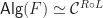
If a monad is of the form $R \circ L$ as in the discussion above, it is referred to as the algebraically free monad over $F$ . We can now state the main facts that we need:

If $\mathbb{T}$ is the algebraically free monad over $F$ , then it is the free monad over $F$ .
If $\mathcal{C}$ is a complete category, and for endofunctor $F : \mathcal{C} \rightarrow \mathcal{C}$ , $F^*$ exists, then the forgetful functor $\mathsf{Alg}(F) \rightarrow \mathcal{C}$ has a left adjoint, and $\mathcal{C}^\mathbb{F^*} \simeq \mathsf{Alg}(F)$ .

So in the case of $\mathsf{Set}$ monads, as the base category is complete, we can reduce the task of finding free monads to that of finding algebraically free monads.

To exploit this connection, we note that every algebraic signature $\Sigma$ induces a signature endofunctor, which we shall also write as $\Sigma : \mathsf{Set} \rightarrow \mathsf{Set}$ . This functor is given by the follow coproduct:

$\Sigma(X) = \coprod_{o \in \Sigma} X^{\mathsf{ar}(o)}$

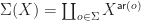
where $\mathsf{ar}(o)$ denotes the arity of operation symbol $o$ .

Example: Let $\Sigma$ be a signature with a single binary operation and a constant. Then the corresponding endofunctor is:

$\Sigma(X) = X \times X + 1$

A $\Sigma$ -algebra is simply a pair $(A, a : A \times A + 1 \rightarrow A)$ . The function $a$ is equivalent to giving a binary function $A \times A \rightarrow A$ , corresponding to the binary operation symbol, and an element of $A$ , corresponding to the constant element. That is the same thing as specifying an algebra for the signature $\Sigma$ .

More generally, it is hopefully clear that for a signature $\Sigma$ , there is an isomorphism between the category of algebras for that signature, and the category of endofunctor algebras for the corresponding signature functor.

For a fixed signature, the free algebra over a set $X$ exists, and is given by the set of all $\Sigma$ -terms over $X$ . From the isomorphism above, this means that the left adjoint to the forgetful functor $\mathsf{Alg}(\Sigma) \rightarrow \mathsf{Set}$ exists, and so therefore does the free monad over $\Sigma$ , with $\Sigma^*(X)$ is the set of all terms over the signature. As usual, it is important to consider examples:

Example: As we have seen in earlier posts, the exception monad $(-) + E$ is induced by an equational presentation with a signature consisting of just constant elements for each exception, and no equations. The signature functor is then the constant functor $K_E$ , and so as we saw earlier, the exception monad is the free monad over this functor.

Example: Consider a signature with a single binary operation. This induces a functor:

$\Sigma(X) = X \times X$

For the free monad over this functor, if we write $+$ for the binary operation, the set $\Sigma^*(X)$ consists of terms such as

$x, x_1 + x_2, (x_1 + x_2) + (x_3 + x_4), \ldots$

We can identify these with binary trees, with the leaves labelled by elements of $X$ . So we have constructed a binary tree monad as the free monad over $(-) \times (-)$ .

Example: Extending the previous example, for an arbitrary signature $\Sigma$ , the resulting free monad will have $\Sigma^*(X)$ consisting of trees such that:

The leaves are labelled with elements of $X$ , or constant symbols from the signature.
The internal nodes of arity $n$ are labelled with an operation symbol of the same arity.

Of course, we could consider $\mathsf{Set}$ endofunctors that are not of the form of signature functors. There are certainly plenty of examples where the left adjoint we require exists. In order to get a concrete description of the induced monad, we would need an explicit description of these adjoints. This requires more technical machinery than we have had chance to introduce so far, so we shall defer this topic to a later post.

Ideal Monads

The free monad constructions in the previous section have some nice properties. If we fix an algebraic signature, and consider the free monad over the corresponding signature functor, as we observed, the elements of $\Sigma^*(X)$ can be thought of as certain labelled trees. Looking a bit more carefully:

The trees in the image of the monad unit are the trivial trees with just a leaf labelled by some element of $X$ .
The functor action $\Sigma^*(h)$ just relabels the leaves of trees, according to the function $h$ .
The functor $\Sigma^*$ can be restricted to the non-trivial trees, as these are preserved by the functor action. We shall denote this functor $\Sigma^+$ .
There is a natural isomorphism $\Sigma^*(X) \cong X + \Sigma^+(X)$ .
Using this isomorphism, the monad unit is the left coproduct injection.
The monad multiplication restricts to non-trivial terms as a natural transformation $\mu' : \Sigma^+ \circ \Sigma^* \Rightarrow \Sigma^+$ in the sense that $\mu \circ \kappa_2 \Sigma^* = \kappa_2 \circ \mu'$ .

So free monads “keep the variables separate” in a well behaved way. The categorical structure above allow us to separate the variables from the non-trivial terms. We now abstract these observations to recover another well-studied class of monads.

An ideal monad is a monad $(\mathbb{T},\eta,\mu)$ such that:

There exists an endofunctor $\mathbb{T}^+$ with $\mathbb{T} = \mathsf{Id} + \mathbb{T}^+$ .
The unit is the left coproduct injection.
There exists $\mu' : \mathbb{T}^+ \circ \mathbb{T} \Rightarrow \mathbb{T}^+$ such that $\mu \circ \kappa_2 \mathbb{T} = \kappa_2 \circ \mu'$ .

Example: Free monads are ideal monads. This is clearly true for those induced by signature functors as discussed above, but in fact this result holds for free monads yielded by more general constructions.

Obviously there would be no need for a separate notion if the only examples were free monads.

Example: The list monad we have discussed previously restricts to a non-empty list monad, and this monad is ideal. The list monad is not ideal. If we consider the list monad as the free monoid monad, we can see this algebraically, as $x = x * 1$ , so the unit is not a coproduct injection. Similarly, the non-ideal multiset monad restricts to the non-empty multiset monad, which is ideal.

We do need to be a little bit careful though. The non-empty finite powerset monad is not ideal. Algebraically this monad is the free join semilattice (without unit element) monad. The idempotence equation $x = x \vee x$ then ensures the monad unit cannot be a coproduct injection.

Algebraically, the ideal monads are the ones where no non-trivial equation of the form $x = t$ is provable, as we have seen in the example above.

There are other interesting classes of ideal monads, making conceptual use of this idea of being able to separate the non-trival terms from the variables. These examples are a whole topic in themselves, and we shall reserve them for a later post.

Further background: For those interested in the mathematics of free monads, a good place to start is the final chapter of Barr and Well’s book “Toposes, Triples and Theories”. A good source for background on ideal monads is Ghani and Uustalu’s paper “Coproducts of Ideal Monads”.

Acknowledgements: Ralph Sarkis pointed out several typos in a previous version of this post, which has greatly improved the content.

Monad bits and pieces

Previous posts have focussed quite a lot on general theory. In this post, we are going to examine a couple of specific monads in a fair amount of detail. Both can be seen as dealing with computations parameterised by a notion of external state.

The Reader or Environment Monad

For any set $R$ , there is a monad with:

Endofunctor: The monad endofunctor is $(-)^R$ .
Unit: The unit at $X$ maps its input to the constant function $x \mapsto (\lambda r.\; x)$ .
Multiplication: The multiplication acts as follows $\mu_X(f)(r) = f(r)(r)$ .

This monad is called the reader or environment monad. The computational interpretation of this monad is that a function $X \rightarrow Y^R$ produces an output that depends on some state or environment it can read. Note the environment is fixed, computations cannot make modifications to it – this will be addressed later.

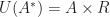
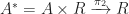
Aside: This monad arises via an adjunction involving slice categories. There is an obvious forgetful functor $U : \mathsf{Set} / R \rightarrow \mathsf{Set}$ . This has a right adjoint $(-)^*$ , with action on objects $A^* = A \times R \xrightarrow{\pi_2} R$ . In turn, this functor has a further right adjoint $\Pi$ . The composite $\Pi \circ (-)^*$ induces the reader monad.

At this level of abstraction, it is not immediately obvious that this adjunction induces the right monad. To at least convince ourselves that the endofunctors agree, we note there is then a series of bijections between hom sets:

$A \rightarrow \Pi(B^*)$
$A^* \rightarrow B^*$
$U(A^*) \rightarrow B$

We then note that $U(A^*) = A \times R$ , and via Cartesian closure functions $A \times R$ bijectively correspond to functions $A \rightarrow A^R$ . Therefore, $\Pi \circ (-)^* \cong (-)^R$ . (The abstract argument generalises well beyond $\mathsf{Set}$ ).

Our main interest is to consider the reader monad from an algebraic perspective. To keep things as simple as possible, we are going to choose $R = \{ 0, 1 \}$ . So computations have access to a single binary bit of external data, which can be set low (0) or high (1). As usual, we would like to have an algebraic presentation of this monad. It is natural to introduce a binary lookup operation $\mid$ , such that informally we interpret

$x \mid y$

as a computation which lookups up what to do depending on the environment value, continuing as $x$ if the bit is low, or $y$ if it is high. We now need to identify some suitable equational axioms that this operation should respect. An immediate idea is to require the operation to be idempotent, that is

$x \mid x \;=\; x$

Intuitively, if we do $x$ regardless of whether the environment bit is high or low, that is the same as behaving exactly as $x$ . A second axiom that springs to mind is:

$(w \mid x) \mid (y \mid z) \;=\; w \mid z$

Here the idea is that:

If the bit is low, we will act as the left component of the left component.
If the bit is high, we will act as the right component of the right component.

In fact, it will turn out that these two axioms are exactly what we need. A simple consequence of the axioms is that:

$x \mid (y \mid z) \;=\; (x \mid x) \mid (y \mid z) \;=\; (x \mid z) \;=\; (x \mid y) \mid (z \mid z) \;=\; (x \mid y) \mid z$

So the operation $|$ is associative. So we can now avoid the annoyance of writing brackets everywhere. We also notice that:

$x \mid y \mid z \;=\; x \mid y \mid z \mid z \;=\; x \mid z$

From the above equations, if we see a sequence of $\mid$ operations, we can eliminate everything but the end points. Combining this with idempotence, it is hopefully not two hard to convince yourself that every term is equal to a unique term of the form $x \mid y$ . So the equivalence classes of terms over $X$ can be identified with pairs of elements from $X$ , equivalently elements of $X^{\{ 0, 1\}}$ .

Finally, we note that

$x \mid y \mid x \;=\; x \mid x \;=\; x$

In fact, the following are equivalent for a structure over a binary operator $\mid$ :

The equations $x \mid x \;=\; x$ and $(w \mid x) \mid (y \mid z) \;=\; w \mid z$ hold.
The equations $x \mid (y \mid z) \;=\; (x \mid y) \mid z$ and $(x \mid y) \mid x \;=\; x$ hold.

For the bottom to top direction, using associativity to ignore brackets:

$x \mid z \;=\; x \mid y \mid x \mid z \mid y \mid z \;=\; x \mid y \mid z$

Using this ability to insert arbitrary elements twice, we calculate:

$w \mid z \;=\; w \mid x \mid z \;=\; w \mid x \mid y \mid z$

Finally, to show idempotence, reusing the first equation we proved:

$x \;=\; x \mid y \mid x \;=\; x \mid x$

The first set of equations we derived from computational intuitions, the second set of equations identify these structures as naturally occurring algebraic objects known as rectangular bands. (A band is an associative idempotent binary operation.) So the Eilenberg-Moore category of the reader monad on a bit is the category of rectangular bands and their homomorphisms.

The State Monad

We have already encountered the state monad, as the monad induced by the Cartesian closed structure on $\mathsf{Set}$ . More precisely, we should refer to this as the global state monad.

Explicitly, for a fixed set of states $S$ , this monad has:

Endofunctor: $S \Rightarrow (- \times S)$ .
Unit: $\eta_X(x)(s) = (x,s)$ .
Multiplication: $\mu_X(f)(s) = \mathsf{let}\; (g,s') = f(s) \; \mathsf{in} \; g(s')$ .

Again, we are going to keep things as simple as possible, and consider a one bit state space, so $S = \{ 0, 1 \}$ . We would like to find an equational presentation for this monad. An obvious place to start is to extend the presentation for the one bit reader monad above, which gives us the infrastructure to decide how to proceed based on the current state. A natural next step is to add operations to manipulate the bit. We could add two unary update operations, say with $\mathop{\uparrow}(x)$ and $\mathop{\downarrow}(x)$ meaning set the state high (low) and proceed as $x$ . We can actually make do with a single bit flip operation, which we shall denote $\mathop{\updownarrow}(x)$ with the intuitive reading of flip the state to its opposite value, and proceed as $x$ . We quickly note that we can define:

$\mathop{\uparrow}(x) \;:=\; \mathop{\updownarrow}(x) \mid x \quad\mbox{ and }\quad \mathop{\downarrow}(x) \;:=\; x \mid \mathop{\updownarrow}(x)$

So the explicit bit setting operations are definable by only flipping the bit if it is the wrong value. Obviously, we expect that

$\mathop{\updownarrow}\mathop{\updownarrow}(x) = x$

as flipping the bit twice should leave us back where we started. We also expect flipping a bit to reverse how computation proceeds:

$\mathop{\updownarrow}(x \mid y) = \mathop{\updownarrow}(y) \mid \mathop{\updownarrow}(x)$

In fact, these equations give a presentation of the one bit state monad. Using the chosen equations, every term is equal to one of the form

$s \mid t$

where both $s$ and $t$ are either a variable, or of the form $\mathop{\updownarrow}(x)$ . This encodes a function taking a bit, saying left or right, and return a variable, and applying a flip to the state if appropriate. That is, an element of $\{ 0, 1 \} \Rightarrow X \times \{ 0, 1 \}$ .

Generalising

To be more realistic, we really should consider larger state spaces or environments. Algebraically, this means instead of a binary lookup operation $\mid$ specifying which of two choices to take depending on a bit value, for an environment with $n$ possible values, we require an $n$ -ary operation. As infix notation is no longer appropriate, we shall write lookup as:

$l(x_1,\ldots,x_n)$

The two axioms that induce the reader monad are the obvious extensions of those for a binary bit.

You may be wondering what to do if the environment is infinite in size. There are well-defined generalisations of universal algebra where operations of these bigger arities are permitted. As long as the maximum size of the operations is bounded, this all pretty much works as in the finite case, so we shall stick with that to keep the notation clearer.

For the state monad, we also need to think about how to change the state. Generalising the bit flip operation seems unnatural, for example should we rotate through the states in some arbitrary order? A better choice is to make the update operations primitive. Without loss of generality, it is notationally convenient to fix a state space $S = \{1,\ldots,n\}$ of natural numbers. We introduce a unary operation $u_i$ for each $i \in S$ . The intuitive reading is that $u_i(x)$ updates the state to $i$ and continues as $u$ . The equations we require, with their intuitive readings are:

$l(u_1(x),\ldots, u_n(x)) = x$ . If we don’t depend on the state, we can ignore it.
$l(l(x_{1,1},\ldots,x_{1,n}),\ldots,l(x_{n,1},\ldots,x_{n,n})) = l(x_{1,1},\ldots,x_{n,n})$ . If the state isn’t modified, we keep making the same choices.
$u_i(u_j(x)) = u_j(x)$ . A second state change overwrites the first.
$u_i(l(x_1,\ldots,x_n)) = u_i(x_i)$ . Update decides a subsequent lookup.

You may have expected the first axiom to be

$l(x,\ldots,x) = x$

In fact, this equation is derivable using the first two. The binary case is:

$x = l(u_1(x), u_2(x)) = l(l(u_1(x), u_2(x)),l(u_1(x),u_2(x))) = l(x,x)$

The general calculation is just notationally a bit harder to read.

The equations above appear in “Notions of Computation Determine Monads” by Plotkin and Power. In fact, they consider a further generalisation, reflecting a more realistic computational setting. We now consider a situation in which we have a set of memory addresses $A$ , and each state has its own independent state value.

If we assume each memory location can take $n$ possible values, we require an $n$ -ary lookup operation $l_a$ for each $a \in A$ , and update operations $u_{a,i}$ , intuitively setting address $a$ to value $i$ . We require the previous equations for each address:

$l_a(u_{a,1}(x),\ldots, u_{a,n}(x)) = x$ . If we don’t depend on the state at an address, we can ignore it.
$l_a(l_a(x_{1,1},\ldots,x_{1,n}),\ldots,l_a(x_{n,1},\ldots,x_{n,n})) = l_a(x_{1,1},\ldots,x_{n,n})$ . If the state at an address isn’t modified, we keep making the same choices when looking up at that address.
$u_{a,i}(u_{a,j}(x)) = u_{a,j}(x)$ . A second state change at the same address overwrites the first.
$u_{a,i}(l_a(x_1,\ldots,x_n)) = u_{a,i}(x_i)$ . Update decides a subsequent lookup at the same address.

We also require some additional axioms, which encode that the states at different addresses don’t interfere with each other.

$l_a(l_{a'}(x_{1,1},\ldots,x_{1,n}),\ldots,l_{a'}(x_{n,1},\ldots,x_{n,n})) = l_{a'}(l_a(x_{1,1}, \ldots, x_{1,n}),\ldots,l_a(x_{1,n},\ldots,x_{n,n}))$ where $a \neq a'$ . Choices based on different addresses commute with each other.
$u_{a,i}(u_{a',j}(x)) = u_{a',j}(u_{a,i}(x))$ where $a \neq a'$ . Consecutive updates at different addresses commute with each other.
$u_{a,i}(l_{a'}(x_1,\ldots,x_n)) = l_{a'}(u_{a,i}(x_1),\ldots, u_{a,i}(x_n))$ where $a \neq a'$ . Updates and lookups at different addresses commute with each other.

The resulting monad is the state monad on $A \times \{ 1,\ldots,n \}$ . Although the algebraic perspective on the reader and state monads was somewhat involved, this does pay off. For example, we now have the data needed to introduce algebraic operations and effect handlers for these monads.

As usual, there are lots more details to take care of in realistic work, such as moving beyond the category $\mathsf{Set}$ , but the underlying intuitions transfer well. Interested readers should read the Plotkin and Power paper mentioned above, which also covers more advanced topics, such as a monad for local state.

The ins and outs of monads

In previous posts we have seen a lot of the basic mathematical infrastructure of monads. The aim of this post is to adopt a computational view on monads, viewing $\mathbb{T}(X)$ as effectful computations over an object $X$ . From this perspective, we shall consider two natural questions:

How can we build such computations? In other words, how do we get things into $\mathbb{T}(X)$ ?
What can we do with computations once have have built them? In other words, how to we get things back out of $\mathbb{T}(X)$ ?

There is a lot of discussion of these topics in the literature. As usual, we will try and keep things simple, restricting attention to simple monads on $\mathsf{Set}$ , and concentrating on the key ideas.

Building computations

So far, the only way have have seen to build elements of $\mathbb{T}(X)$ is to apply the monad unit $\eta_X$ .

Example: For the exception monad, for set of exceptions $E$ , the value $\eta(x) = (1,x) \in X + E$ is a trivial computation that returns the value $x$ , and doesn’t throw an exception.

Example: The finite powerset monad $\mathbb{P}$ can be seen as a form of bounded non-determinism. $\eta(x) = \{ x \} \in \mathbb{P}(X)$ is a trivially non-deterministic computation that always results in the value $x$ .

Example: The list monad $\mathbb{L}$ can be seen as a form of non-determinism which can be easier to implement in a programming language. It is unusual as there is an order on computations, and repeated values are allowed. Obviously another perspective is to see such computations as living in a list data structure. Again $\eta(x) = [x]$ is the trivial singleton list containing only the value $x$ .

The intuition we derive from these examples is that $\eta(x)$ yields a trivially effectful computation in some suitable sense. To get any real use out of these computational effects, we need to be able to build less boring examples as well. To solve this problem, as usual we shall adopt an algebraic perspective. Assume we have an equational presentation $(\Sigma, E)$ . An $n$ -ary operation $o \in \Sigma$ induces a function $\mathbb{T}^n(X) \mapsto \mathbb{T}(X)$ as follows:

$([t_1],\ldots,[t_n]) \mapsto [o(t_1,\ldots,t_n)]$

Continuing the examples above:

Example: The exception monad has a presentation consisting of a constant $e$ for each exception in $E$ . These induce functions $\mathsf{raise}_e : 1 \rightarrow \mathbb{X}$ with action $\star \mapsto e$ , which we can think of as raising the exception $e$ .

You may wonder where the notion of catching or handling an exception appears. This is a good question, and will be addressed in the next section.

Example: The finite powerset monad has a presentation with a binary operation $\vee$ and a constant element $\bot$ . The constant induces a function $\bot : 1 \rightarrow \mathbb{P}(X)$ with action $\star \mapsto \emptyset$ , which we can think of as picking out a diverging computation.

The binary operation induces an operation $\vee : \mathbb{T}(X)^2 \rightarrow \mathbb{X}$ with action $(U,V) \mapsto U \cup V$ , which takes two non-deterministic computations, and combines their possible behaviours. For example $\eta(x_1) \vee \eta(x_2)$ is a computation yielding either $x_1$ or $x_2$ .

Example: Similarly to the previous example, the list monad has a presentation with binary operation $\times$ , and a constant element $1$ . The constant induces a function $1 \rightarrow \mathbb{T}(X)$ with action $\star \mapsto []$ .

The binary operation induces a function $\mathbb{T}(X)^2 \rightarrow \mathbb{T}(X)$ with action $([x_1,\ldots,x_m],[x_{m + 1}, \ldots, x_{n}]) \mapsto [x_1,\ldots,x_n]$ concatentating two lists. We can interpret these operations as simply manipulating data structures, or more subtly as a form of non-determinism in which the operations respect the order on choices.

Rather than describe these operations directly in terms of substitutions, it would be better to phrase things in terms of the available monad structure. To do so, we abuse notation and let $m$ denote the set $\{1,\ldots,m \}$ . A family of $m$ equivalence classes of terms over $X$ , $([t_i])_{1 \leq i \leq m}$ , can be identified with a morphism $t: m \rightarrow \mathbb{T}(X)$ , and a single $m$ -ary term with a map $o : 1 \rightarrow \mathbb{T}(m)$ . The composite $t^* \circ o : 1 \mapsto \mathbb{T}(X)$ , where $t^*$ denotes the Kleisli extension of $t$ , corresponds to the substitution we are interested in:

$([t_1],\ldots,[t_n]) \mapsto [o(t_1,\ldots,t_n)]$

In fact, we have generalised slightly, as $o$ is now an arbitrary term, not just an operation appearing in the signature.

Of course, we expect these mapping $\mathbb{T}(X)^n \rightarrow \mathbb{T}(X)$ induced by Kleisli morphism to behave in a suitably uniform way. That is, they should be natural in some sense. This actually requires a modicum of care to get right. We should really consider our mapping as being of type $U_{\mathbb{T}}(X)^n \rightarrow U_{\mathbb{T}}(X)$ . Here, $U_{\mathbb{T}} : \mathsf{Set}_{\mathbb{T}} \rightarrow \mathsf{Set}$ is the forgetful functor from the Kleisli category. This has action on objects $X \mapsto \mathbb{T}(X)$ , so this rephrasing makes sense. We then note that the induced maps:

$U_{\mathbb{T}}^n(X) \rightarrow U_{\mathbb{T}}(X)$

are natural. This is sometimes phrased as being natural with respect to Kleisli morphisms. They also trivially interact well with the strength morphisms in $\mathsf{Set}$ . In more general categories, there is a bijection between:

Families of morphisms $U_{\mathbb{T}}^n(X) \rightarrow U_{\mathbb{T}}(X)$ Kleisli natural in $X$ , and interacting well with monad strength. These are referred to as algebraic operations.
Morphisms $1 \rightarrow \mathbb{T}(m)$ , referred to as generic effects.

To give a denotational semantics for a serious programming language, a lot more details need filling in. The category $\mathsf{Set}$ is not suitable for realistic work, but is certainly a helpful way to build up the basic intuitions.

Evaluating computations

Now we have some tools for building up elements of $\mathbb{T}(X)$ , what can we do with them? The unit and multiplication of a monad have types $\mathsf{Id} \Rightarrow \mathbb{T}$ and $\mathbb{T}^2 \Rightarrow \mathbb{T}$ , so so they give us no way “out of the monad”.

What we are looking for is a systematic way of building well-behaved maps of type $\mathbb{T}(X) \rightarrow Y$ for some $Y$ . The key idea is to recall the Eilenberg-Moore adjunction. For a set $X$ , the free algebra over $X$ is:

$F^{\mathbb{T}}(X) = (\mathbb{T}(X), \mu_X)$

The universal property of this adjunction means that if we can identity another Eilenberg-Moore algebra $(Y,\xi)$ , and a homomorphism

$h : X \rightarrow Y$

these bijectively corresponds to algebra homomorphisms:

$F^{\mathbb{T}}(X) \xrightarrow{\hat{h}} (Y,\xi)$

That is, morphisms

$\mathbb{T}(X) \rightarrow Y$

respecting the algebraic structure. It is worth considering the roles of these components:

The homomorphism $h : X \rightarrow Y$ specifies how values should be interpreted.
The algebra $(Y, \xi)$ specifies how the structure used to build up an effectful computation should be evaluated, in a manner respecting the structure encoded by the monad.

As usual, this is probably best understood by considering some examples.

Example: For the exception monad over $E$ , an Eilenberg-Moore algebra $(Y, \xi : Y + E \rightarrow Y)$ must act as the identity on the left component of the coproduct, and send each element of the right component to any value of its choosing in $Y$ . In other words, we specify a default value to take for each of the exceptions that might be raised. Given a function $h : X \rightarrow Y$ , the induced algebra morphism will map values according to $h$ , and otherwise chose the value specified by $\xi$ when it encounters a raised exception.

Example: For the finite powerset monad $\mathbb{P}$ , giving an Eilenberg-Moore algebra is equivalent to specifying a join semilattice structure. For example, we can consider the Eilenberg-Moore algebra on the natural numbers $\mathbb{N}$ specified by taking the maximum of pairs of elements, and bottom value $0$ . The resulting homomorphism $\mathbb{P}(\mathbb{N}) \rightarrow \mathbb{N}$ induced by the identity will map a finite set to its maximum value (inevitably defaulting to $0$ if the set is empty).

Example: The pattern for the list monad is similar. An Eilenberg-Moore algebra is a monoid, so we must specify a multiplication and unit element. For example if $X$ is the set of two by two matrices over the natural numbers, this carries a monoid structure under matrix multiplication. The identity on $X$ then induces a map $\mathbb{L}(X) \rightarrow X$ that multiplies a list of matrices together from left to right. Note that this example fundamentally exploits the fact that the multiplication operation is not forced to be commutative.

The ideas in this section are the basics of what are known as effect handlers. As with algebraic operations, to produce a denotational semantics for a realistic programming language, and more complex handlers, there are many details to take care of, and we must move beyond $\mathsf{Set}$ . However, this simplified setting is sufficient to illustrate the key ideas, without dealing with distracting technical details.

Summary

We have have seen the basic mathematical machinery to build effectful computations within a monad, and also how to evaluate these computation to values. The main points are:

The morphisms that allow us to build elements of $\mathbb{T}(X)$ arise naturally from an algebraic presentation of the monad.
The morphisms that allow us to evaluate computations in $\mathbb{T}(X)$ require us to make choices as to how that evaluation should proceed, specifically a suitable Eilenberg-Moore algebra, and then exploit the universal property of free algebras.

The literature in this area contains many nice examples, and is enjoyable to read. For algebraic operations and generic effects, search for work of Plotkin and Power, and for effect handlers, the work of Pretnar, Plotkin and Bauer are good places to start reading. There is a lot more to these topics than the details we have sketched here, so it is well worth exploring further.

We have also been limited in our example by the relatively simple monads we have introduced so far. We will see more interesting monads from a computational perspective in later posts.

Commutativity Algebraically

Recall the substitution notation we have been using:

$t[t_x / x \mid x \in X]$

denotes the term $t$ , with each $x \in X$ simultaneously replaced by the term $t_x$ . For an equational presentation $(\Sigma, E)$ , inducing a monad $\mathbb{T}$ , consider a pair:

$([s],[t]) \in \mathbb{T}(X) \times \mathbb{T}(Y)$

where $[t]$ denotes an equivalence class with representative term $t$ . We can then write the action of the first double strength map in terms of representatives and substitutions as:

$\mathsf{dst}([s],[t]) = [t[s[(x,y)/x \mid x \in X] / y \mid y \in Y]]$

and the second:

$\mathsf{dst}'([s],[t]) = [s[t[(x,y)/y \mid y \in Y] / x \mid x \in X]]$

Therefore, the resulting monad is commutative if and only if for all $s,t$ , the following equality is provable in equational logic:

$t[s[(x,y)/x \mid x \in X] / y \mid y \in Y] = s[t[(x,y)/y \mid y \in Y] / x \mid x \in X]$

We shall call this the commutativity condition.

The substitutions can be made a bit easier to read with a change of notation. For two terms $s,t$ , let $x_1,\ldots,x_m$ and $y_1,\ldots,y_n$ be a choice of enumeration of the variables appearing in the two terms. We can then write them as

$s(x_1,\ldots, x_m) \quad\mbox{ and }\quad t(y_1,\ldots,y_n)$

and writing substitution in the natural way, the commutativity condition becomes:

$t(s((x_1,y_1),\ldots,(x_m,y_1)),\ldots, s((x_1,y_n),\ldots,(x_m,y_n))) = s(t((x_1,y_1),\ldots,(x_1,y_n)),\ldots,t((x_m,y_1),\ldots,(x_m,y_n)))$

That’s an awful lot of formal notation and brackets to deal with. Let’s consider some implications of this condition to build intuition for what it means in practice.

Example: Consider a presentation with binary operations $+$ and $\times$ . The action of the double strengths on $[x + x'] \in \mathbb{T}(X)$ and $[y \times y'] \in \mathbb{T}(Y)$ are:

$\mathsf{dst}([x + x'], [y \times y']) = [((x,y) + (x',y)) \times ((x,y') + (x',y'))]$

and

$\mathsf{dst}'([x + x'], [y \times y']) = [((x,y) \times (x,y')) + ((x',y) \times (x',y'))]$

If the monad $\mathbb{T}$ is commutative, the following equality must be provable in equational logic:

$((x,y) + (x',y)) \times ((x,y') + (x',y')) = ((x,y) \times (x,y')) + ((x',y) \times (x',y'))$

As a special case of this observation, any monad presented by a binary operation must satisfy the following equation:

$((x,y) + (x',y)) + ((x,y') + (x',y')) = ((x,y) + (x,y')) + ((x',y) + (x',y'))$

If $+$ is associative, this boils down to:

$(x,y) + (x',y) + (x,y') + (x',y') = (x,y) + (x,y') + (x',y) + (x',y')$

The only difference between the two terms is the order of the middle two constants, so this equality will certainly hold for any associative commutative binary operation. This condition is satisfied in many natural algebraic structures, and does exhibit a very weak relationship between commutative operations and commutative monads.

An instructive boundary case is the following.

Example: Consider two terms $s,t$ in which no variables appear. These are constants in our equational theory. The commutativity condition implies that:

$s = t$

as all the variable substitutions become trivial. Therefore any equational presentation of a commutative monad can have at most one distinct constant term. We have already encountered this phenomenon. The exception monad is only commutative when there is at most one exception constant.

“Constant counting” can be a quick way to discount the possibility that a monad for an equational presentation is commutative. For example the monads corresponding to commutative rings or rigs (semirings) cannot be commutative as they have distinct constant symbols for the additive and multiplicative structures. These are further natural examples of monads with all the binary operations in the signature commutative, but the resulting monads are not commutative.

Another simple case is worth considering.

Example: Let $s \in \mathbb{T}(X)$ and $t \in \mathbb{T}(Y)$ be terms in which only one variable appears, say $x_0$ and $y_0$ respectively. Then the left hand side of the commutativity condition is:

$t[s[(x,y)/x \mid x \in X] / y \mid y \in Y] = t(s((x_0,y_0)))$

and the right hand side is:

$s[t[(x,y)/y \mid y \in Y] / x \mid x \in X] = s(t((x_0,y_0)))$

So for $\mathbb{T}$ to be commutative, each pair of unary terms must satisfy $s(t(x)) = t(s(x))$ .

As an application of this special case, we introduce another commonly considered monad. For a fixed monoid $(M,\times,1)$ the writer monad has:

Endofunctor: The endofunctor is the product $M \times (-)$ .
Unit: $\eta(x) = (1,x)$ .
Multiplication: $\mu(m,(n,x)) = (m \times n, x)$ .

Computationally, this monad can be seen as encoding computations that also record some additional output such as logging. The monoid structure combines the outputs from successive computations. Algebraically, it corresponds to actions of the monoid $M$ .

The writer monad has an equational presentation with one unary operational symbol for each element of the monoid, and equations:

$1(x) = x$ .
$p(q(x)) = r(x)$ if and only if $p \times q = r$ in the monoid.

Using our observation above, the writer monad is commutative if and only if the monoid $M$ is commutative. So in this case, we do see a strong connection between the monadic and algebraic notions of commutativity.

Another useful boundary case is to consider what the commutativity condition means for variables.

Example: Consider a variable $x_0$ and an an arbitrary term $t$ . The left hand side of the commutativity condition is:

$t[x_0[(x,y)/x \mid x \in X] / y \mid y \in Y] = t[(x_0,y) \mid y \in Y]$

and the right hand side is:

$x_0[t[(x,y)/y \mid y \in Y] / x \mid x \in X] = t[(x_0,y) \mid y \in Y]$

So variables always satisfy the commutativity condition with respect to any other term. With hindsight, maybe we should not find this too surprising.

We will now consider an important example, which will point the way to getting a better handle on the unpleasant looking general commutativity condition we deduced above.

Example: We now consider an equational presentation with a constant term $0$ and a binary term $x + x'$ and a unary term $h$ . The equations yielded by the commutativity condition for the pairs $([h],[0])$ and $([h],[x + x'])$ are:

$h(0) = 0 \quad\mbox{ and }\quad h((x,y) + (x',y)) = h((x,y')) + h((x',y'))$

we can simplify the second condition by renaming variables, and we arrive at the conditions:

$h(0) = 0\quad\mbox{ and }\quad h(x + x') = h(x) + h(x')$

These conditions should hopefully look familiar, they are exactly the equations we require for $h$ to be a homomorphism with respect to $+$ and $0$ .

We now aim to make the connection with homomorphisms from the previous example precise by making two observations:

For positive natural $k$ and set $Z$ , the term $s(x_1,\ldots,x_m)$ induces an $m$ -ary operation on $\mathbb{T}^k(Z)$ with action $(([t_{1,1}],\ldots,[t_{1,k}]),\ldots,([t_{m,1},\ldots,t_{m,k}])) \mapsto ([s(t_{1,1},\ldots,t_{m,1})],\ldots,[s(t_{1,k},\ldots,t_{m,k})])$ .
Similarly, the term $t(y_1,\ldots,y_m)$ induces an $n$ -ary function $\mathbb{T}(Z)^{n} \rightarrow \mathbb{T}(Z)$ with action $([t_1],\ldots, [t_n]) \mapsto [t(t_1,\ldots,t_n)]$

The homomorphism condition is equivalent to saying that the $n$ -ary function $\mathbb{T}(X \times Y)^{n} \rightarrow \mathbb{T}(X \times Y)$ induced by $t$ is a homomorphism with respect to the $m$ -ary operation induced by $s$ . In this sense, the commutativity conditions can be rephrased as all the terms are homomorphisms with respect to each other.

From the algebraic perspective a monad is commutative in the sense that all terms can be commuted past each other as homomorphisms.

Being commutative has nothing to do with being commutative

In explanations about commutative monads, it is common to see a passing remark such as “as we’d expect, the Abelian monoid monad is commutative”. Now I might be over-interpreting these comments, but they seem to imply that the monad being commutative is related to the algebraic structure having a commutative binary operation. Now it is true that the Abelian monoid (a.k.a. multiset) monad is commutative, and several other commutative monads are induced by algebraic structures with commutative binary operations, but how well does this intuition hold together more generally?

Firstly, we consider if being a commutative monad implies commutativity of the binary operations in equational presentations.

Counterexample: We saw last time that the finite distribution monad is commutative. This monad is isomorphic to the monad presented by a family of binary operations $\{+^r \mid r \in (0,1) \}$ satisfying the following equations:

Idempotence: For all $r \in (0,1)$ , $x +^r x = x$ .
Pseudo-commutativity: For all $r \in (0,1)$ , $x +^r y = y +^{1 - r} x$ .
Pseudo-associativity: For all $r,s \in (0,1)$ , $x +^r (y +^s z) = (x +^{\frac{r}{r + (1-r)s}} y) +^{r + (1-r)s} z$

Algebras for this theory are called convex algebras. Intuitively, the operation $x +^r y$ forms the probabilistic mixture $rx + (1-r)y$ and the axioms can be understood from this point of view. The pseudo-associativity axiom is particularly unpleasant to look at, but is easier to understand in terms of re-bracketing weighted binary combinations.

The axioms presenting convex algebras don’t have explicit commutativity equations for all the binary operations, but they might be derivable. To make sure this isn’t the case, we consider the concrete description of the free algebras that we get from the isomorphism to the finite distribution monad.

Specifically, the free algebra on $X$ has universe finitely supported convex sums over $X$ , and the operations are the obvious weighted sums:

$(\sum_i p_i x_i) +^r (\sum_j q_j y_j) = \sum_i (r \times p_i) x_i + \sum_j ((1-r) \times q_j) y_j$

This operation is clearly not commutative, except when $r = \frac{1}{2}$ . So there is a commutative monad presented by an algebraic theory with (many different) non-commutative algebraic operations.

(I thank Maaike Zwart for suggesting this natural concrete counterexample)

What about the other direction, does an equational presentation where all the binary operations are commutative imply commutativity?

Counterexample: We have already seen that the exception monad $(-) + E$ is only commutative if $E$ is a singleton set. The exception monad is isomorphic to the monad for an equational theory with constant symbols the elements of $E$ , and no equations. So there are both commutative and non-commutative monads with presentations containing no binary operations at all.

The previous counterexample is a bit too trivial to be satisfactory, as there are no binary operations involved at all, and we’re quantifying over the empty set when making statements about commutativity in the algebraic sense.

As a second attempt, we shall synthesise an equational presentation in which the only components involved are commutative binary operations.

Counterexample: Consider an equational presentation with two binary operations $\oplus$ and $\otimes$ , with the only equations being those requiring both operations are commutative. We consider the action of the double strengths on the equivalence classes $[w \oplus x]$ and $[y \otimes z]$ . For the first:

$\mathsf{dst}([w \oplus x], [y \otimes z]) = [((w,y)\oplus(x,y)) \otimes ((w,z)\oplus(x,z))]$

and for the second:

$\mathsf{dst}'([w \oplus x], [y \otimes z]) = [((w,y)\otimes(w,z)) \oplus ((x,y)\otimes(x,z))]$

If this monad is commutative, we must have equality of equivalence classes:

$[((w,y)\oplus(x,y)) \otimes ((w,z)\oplus(x,z))] = [((w,y)\otimes(w,z)) \oplus ((x,y)\otimes(x,z))]$

We note that the provable equalities $t = t'$ in our theory must have the same number of occurrences of $\oplus$ and $\otimes$ on both sides. Therefore the two equivalence classes are distinct, and the monad is not commutative.

So we have seen that there is a monad that is not commutative, presented by an equational theory containing only commutative binary operations.

The previous two counterexamples reflect the fact that commutative binary operations should not have anything essential to do with monad commutativity. Monads presented by theories with just constants may or may not be commutative. Theories just involving just binary operations may or may not be commutative. Obviously there are other arities of operation to consider, but by this point hopefully it’s clear that there’s no tight relationship.

In fact, a monad being commutative does imply that certain equations must hold. In the case of binary operations, it is sufficient for the operation to be commutative to satisfy some of these equations. In simple cases, for example theories with a single binary operation, this might explain some of the misleading patterns that emerge.

We shall examine commutative monads from an algebraic perspective in a later post, and see exactly what it is that can be commuted that inspires the terminology.

Commutative Monads

We saw the two double strength natural transformations in the previous post:

$\mathsf{dst}, \mathsf{dst}' : \mathbb{T}(A) \otimes \mathbb{T}(B) \rightarrow \mathbb(T)(A \otimes B)$

A commutative monad is a strong monad for which $\mathsf{dst} = \mathsf{dst}'$ . We saw last time that the list monad is not commutative, but the powerset monad is. In this post we will restrict ourselves to examining some more instructive examples. This will help build our intuitions, and the examples lay the groundwork for discussions in later posts.

Example: For a set $E$ , there is a monad with:

Endofunctor: $(-) + E$ .
Unit: The unit maps an element into the left component of the coproduct $x \mapsto (1,x)$ .
Multiplication: The multiplication: $\mu_X : (X + E) + E \Rightarrow X + E$ does the “obvious thing”, $(1,(1,x)) \mapsto (1,x)$ , $(1,(2,e)) \mapsto (2,e)$ and $(2,e) \mapsto (2,e)$ .

The monad is sometimes referred to as the exception monad. Computationally, we can interpret a Kleisli morphism $X \rightarrow Y + E$ as a function that transforms elements of $X$ to elements of $Y$ , but may return error or exception values captured by $E$ . The first double strength for this monad is defined by the following cases:

$\mathsf{dst}((1,x), (1,y)) = (1, (x,y))$ .
$\mathsf{dst}((2,e),(1,y)) = (2,e)$ .
$\mathsf{dst}((1,x),(2,e)) = (2,e)$ .
$\mathsf{dst}((1,e_1),(1,e_2)) = (2,e_2)$ .

Notice that exception values are preferred, but there is rather arbitrary choice that has to be made in the fourth case. The second double strength agrees with the first, except for the final case, where it makes the other choice of exception to prefer:

$\mathsf{dst}'((1,e_1),(1,e_2)) = (2,e_1)$ .

So we see that the exception monad is only commutative if there’s exactly one exception. This special case is sometimes referred to as the maybe monad, as computationally it encodes functions that may fail.

Example: The multiset monad is commutative. To describe this, we shall introduce the notation

$\{ x_1 : k_1,\ldots, x_n : k_n \}$

for a multiset where element $x_i$ appears with multiplicity $k_i$ . The action of both double strength maps sends the pair of multisets:

$(\{ x_1 : k_1, \ldots, x_n : k_n \}, \{ y_1 : l_1,\ldots, y_m : l_m \})$

to the multiset:

$\{ (x_i , y_j) : k_i \times l_j \mid 1 \leq i \leq n, 1 \leq j \leq m \}$ .

The multiset monad is (isomorphic to) the Abelian monoid monad, so this monad is also commutative.

Example: Another monad that occurs commonly in practice is the finite probability monad on $\mathsf{Set}$ . This has:

Endofunctor: $\mathbb{D}(X)$ has elements finitely supported formal convex sums $\sum_i p_i x_i$ . These are weighted sum of elements of $X$ such that for each weight $p_i$ , $1 \leq p_i \leq 1$ , $\sum_i p_i = 1$ and only finitely many $p_i$ are non-zero. Alternatively, these can be thought of as functions $X \rightarrow [0,1]$ satisfying the previous conditions on the weights.
Unit: $\eta_X(x) = x$ . That is, the unit maps an element of $X$ to the corresponding trivial sum.
Multiplication: $\mu_X(\sum_i p_i (\sum_j q_{i,j} x_{i,j})) = \sum_i \sum_j (p_i \times q_{i,j}) x_{i,j}$ . This is simply flattening out a sum of sums.

This monad is commutative, with the action of both double strengths being:

$(\sum_i p_i x_i, \sum_j q_j y_j) \mapsto \sum_i \sum_j (p_i \times q_j) (x_i,y_j)$

For example:

$(\frac{1}{4}x + \frac{3}{4}x', \frac{1}{3} y + \frac{2}{3} y') \mapsto \frac{1}{12}(x,y) + \frac{1}{4}(x',y) + \frac{1}{6}(x,y') + \frac{1}{2}(x',y')$

In the next post we will explore a slightly misleading intuition that is commonly hinted at in the literature.

Other Monad Strengths

Last time, we saw the notion of strength for a monad. These were natural transformations

$A \otimes \mathbb{T}(B) \rightarrow \mathbb{T}(A \otimes B)$

which interact well with the monoidal and monad structure. As was mentioned last time, there are other ways we might consider commuting a functor with a monoidal structure. The obvious first choice is to consider a natural transformation of type

$\mathbb{T}(A) \otimes B \rightarrow \mathbb{T}(A \otimes B)$

again, interacting sensibly with the monoidal and monad structure (as before, we leave the details of what this means aside, to concentrate on the main ideas). Such a natural transformation is called a costrength, denoted $\mathsf{st}'$ .

Example: If $\mathcal{V}$ is a symmetric monoidal category we can build a costrength from a strength

$\mathsf{st}_{A,B} : A \otimes \mathbb{T}(B) \rightarrow \mathbb{T}(A \otimes B)$

as the composite:

$\mathbb{T}(A) \otimes B \xrightarrow{\sigma_{\mathbb{T}(A),B}} B \otimes \mathbb{T}(A) \xrightarrow{\mathsf{st}_{B,A}} \mathbb{T}(B \otimes A) \xrightarrow{\mathbb{T}(\sigma_{B,A})} \mathbb{T}(A \otimes B)$

Here $\sigma$ is the symmetry isomorphism from the symmetric monoidal structure. Intuitively, we just swap the inputs, use the strength and swap them back again.

As we know every $\mathsf{Set}$ monad is strong in a unique way, so it also has a unique costrength. For example, the costrength for the list monad acts as follows:

$([a_1,\ldots,a_n],b) \mapsto [(a_1,b),\ldots,(a_n,b)]$

Unsurprisingly, costrength for the powerset is very similar, visually we just swap square (list formation) brackets for curly (set formation) brackets.

$(\{a_1,\ldots,a_n\},b) \mapsto \{(a_1,b),\ldots,(a_n,b)\}$

We can consider costrengths beyond symmetric monoidal categories, as their definition does not require the existence of a strength morphism. In the cases that will be of interest to us, it will be the interplay between strengths and costrengths that will matter. To keep things simple, we will assume we are working in a symmetric monoidal category, so the costrength can be derived from the strength (or vice-versa), as in the example above. (To move beyond this setting, we would need to assume further compatibility conditions between any choice of strength and costrength, which are automatic when one is derived from the other via a monoidal symmetry.)

One we have a strength $\mathsf{st}$ and costrength $\mathsf{st}'$ , we can build a natural transformation of type $\mathbb{T}(A) \otimes \mathbb{T}(B) \rightarrow \mathbb{T}(A \otimes B)$ . In fact, there are two ways we can do this, either by applying strength first:

$\mathsf{dst} = \mathbb{T}(A) \otimes \mathbb{T}(B) \xrightarrow{\mathsf{st}_{A,B}} \mathbb{T}(\mathbb{T}(A) \otimes B) \xrightarrow{\mathbb{T}(\mathsf{st}'_{A,B})} \mathbb{T}^2(A\otimes B) \xrightarrow{\mu_{A \otimes B}} \mathbb{T}(A \otimes B)$

or applying costrength first:

$\mathsf{dst}' = \mathbb{T}(A) \otimes \mathbb{T}(B) \xrightarrow{\mathsf{st}'_{A,B}} \mathbb{T}(A \otimes \mathbb{T}(B)) \xrightarrow{\mathbb{T}(\mathsf{st}_{A,B})} \mathbb{T}^2(A \otimes B) \xrightarrow{\mu_{A \otimes B}} \mathbb{T}(A \otimes B)$

Both these composites are referred to as double strengths. Whenever we see two composites of the same type in category theory, it is natural to consider if they are always the same.

Example: For the list monad, we have:

$\mathsf{dst}([a,b],[c,d]) = [(a,c),(b,c),(a,d),(b,d)]$

whereas

$\mathsf{dst}'([a,b],[c,d]) = [(a,c),(a,d),(b,c),(b,d)]$

notice the difference in the order of the middle two elements.

On the other hand, for the powerset monad, essentially because there is no ordering in subsets:

$\mathsf{dst}(\{a,b\},\{c,d\}) = \mathsf{dst}'(\{a,b\},\{c,d\}) = \{(a,c),(b,c),(a,d),(b,d) \}$

This is not an isolated example, for the powerset monad $\mathsf{dst} = \mathsf{dst}'$ .

The previous examples show us that in general $\mathsf{dst} \neq \mathsf{dst}'$ , but the two composites may agree for some monads. This question, and its implications are another key topic in the theory of monads. We shall begin exploring the details in the next post.

Strong Monads

Strong monads, the topic of this post, are a somewhat technical looking topic at first glance, requiring more definitions and machinery than we have seen up until now. Unfortunately, they are key to some more interesting topics, both mathematically and in terms of computer science application. As usual when dealing with new abstract ideas, it is useful to focus on intuitions and examples to get a feeling for the formal definitions. This post is longer than might be ideal, but there are plenty of examples.

For those interested in the technical details I skip, some recommended reading:

Monoidal categories: “Categories for the Working Mathematician” by Mac Lane has a very readable account of monoidal categories, despite its reputation for requiring a lot of mathematical background.
Enriched categories: Both volume 2 of Borceux’s “Handbook of Categorical Algebra”, and Riehl’s “Categorical Homotopy Theory” have brief introductions to monoidal categories, to set up a concise introduction to enriched category theory. The standard reference for enriched category theory is Kelly’s “Basic Concepts of Enriched Category Theory”, which also contains the necessary background on monoidal categories. This book can be difficult in places, but the material we require is covered at a reasonable pace.

Monoidal Categories

A monoidal category is a category $\mathcal{V}$ with a monoidal product bifunctor, typically denoted $\otimes$ , and a unit object, $I$ . Intuitively, this is a generalization of the notion of monoid from sets to categories. There are isomorphisms

$\lambda : I \otimes A \rightarrow A \qquad \rho : A \otimes I \rightarrow A$ ,

natural in $A$ , and referred to as the left and right unitor respectively. These encode that $I$ acts as a unit for the multiplication, up to isomorphism. There are also associator isomorphisms:

$\alpha : (A \otimes B) \otimes C \rightarrow A \otimes (B \otimes C)$ ,

natural in $A, B, C$ , encoding associativity up to isomorphism. The unitors and associator are required to satisfy some compatibility equations (referred to as coherence conditions). We won’t need the details, but they can be found in any standard category theory reference.

A symmetric monoidal category is a monoidal category with a further symmetry isomorphisms encoding commutativity up to isomorphism:

$\sigma : A \otimes B \rightarrow B \otimes A$

natural in $A,B$ . Again, the symmetry is required to satisfy some coherence conditions (equations) with respect to the other structure. Finally, a (symmetric) monoidal closed category is a (symmetric) monoidal category such that for each object $A$ , there is an adjunction:

$(-) \otimes A \dashv A \multimap (-)$

Example: Any category $\mathcal{C}$ with products is a symmetric monoidal category, with

$A \otimes B = A \times B \qquad I = 1$

The left and right unitors, associator and symmetry are the “obvious” canonical maps induced by the universal property of products. If $\mathcal{C}$ is Cartesian closed, then it is symmetric monoidal closed, with $A \multimap (-)$ given by the exponential $A \Rightarrow (-)$ .

In particular, the category $\mathsf{Set}$ is symmetric monoidal closed with monoidal product given by Cartesian products, and $A \multimap (-)$ given by the function space functor $A \Rightarrow (-)$ . This is the motivating example for much of what follows, and of practical interest in algebraic examples we shall see later. When working with $\mathsf{Set}$ , if not otherwise stated the monoidal structure is taken to be the Cartesian product structure.

Strength

For a monoidal category $\mathcal{V}$ , and endofunctor $T: \mathcal{V} \rightarrow \mathcal{V}$ , a strength (sometimes referred to as a tensorial strength) for $T$ is a natural transformation

$\mathsf{st}_{A,B} : A \otimes T(B) \rightarrow T(A \otimes B)$

which satisfies two coherence conditions with respect to the monoidal structure. A strong functor is a functor with a chosen strength. A strong monad is monad $\mathbb{T}$ with a strong underlying endofunctor, satisfying additional coherence conditions with respect to the monad unit and multiplication. Again, the actual coherence conditions can be found in standard sources, we shall focus on examples and intuitions.

Example: The list and powerset monads are both strong in a unique way, with strengths:

$(a, [b_1,\ldots,b_n]) \mapsto [(a,b_1),\ldots,(a,b_n)]$

$(a, \{ b_1,\ldots, b_n \}) \mapsto \{ (a,b_1), \ldots, (a,b_n) \}$

We shall shortly see that form (and uniqueness) of the strengths for the $\mathsf{Set}$ monads in the previous example are in no way special.

So a crude first sketch of a strength is that it is a well-behaved way of commuting an endofunctor and a monoidal product. You may notice that there are other ways you might imagine commuting an endofunctor with a monoidal product. We shall return to that thought in later posts.

To get a more principled mathematical perspective on strength, unfortunately we need to introduce further abstract machinery.

Enriched Categories

Enriched category theory is a large and potentially complex topic. Fortunately we will only need a few of the basic definitions, and no deep theory. The idea of an enriched category is that often for a category $\mathcal{C}$ , the homsets $\mathcal{C}(A,B)$ carry additional mathematical structure, and this structure interacts well with composition. For example:

Example: The homsets in the category $\mathsf{Pre}$ of preorders and monotone maps actually carry a natural pointwise order:

$f \leq g \Leftrightarrow \forall a. f(a) \leq g(a)$ .

This structure satisfies:

$f_1 \leq f_2 \;\wedge\; g_1 \leq g_2 \quad\Rightarrow\quad g_1 \circ f_1 \leq g_2 \leq f_2$

when the composites are well-defined. So the homsets are actually $\mathsf{Pre}$ -objects, and the composition maps are $\mathsf{Pre}$ -morphisms

$\mathsf{Pre}(B,C) \times \mathsf{Pre}(A,B) \rightarrow \mathsf{Pre}(A,B)$

A close relative of the previous example is the following:

Example: The homsets of the category of all (small) categories $\mathsf{Cat}$ are themselves categories, with morphisms the natural transformations. Furthermore, the composition maps are bifunctors

$\mathsf{Set}(B,C) \times \mathsf{Set}(A,B) \rightarrow \mathsf{Set}(A,C)$

An important trivial example is the following:

Example: The homsets of the category $\mathsf{Set}$ are $\mathsf{Set}$ -objects, and the composition maps are $\mathsf{Set}$ -morphisms

$\mathsf{Set}(B,C) \times \mathsf{(Set}(A,B) \rightarrow \mathsf{Set}(A,B)$

Finally, a slightly different example, which motivates the level of generalization of the formal definition.

Example: The homsets of the category of Abelian groups $\mathsf{Ab}$ can be given the structure of Abelian groups pointwise. With this structure, the composition maps satisfy:

$(g_1 + g_2) \circ f = (g_1 \circ f) + (g_2 \circ f) \qquad 0 \circ f = 0$

and the dual conditions for precomposition. This is not the same as saying the composition maps are $\mathsf{Ab}$ morphisms:

$\mathsf{Ab}(B,C) \times \mathsf{Ab}(A,B) \rightarrow \mathbb{Ab}(A,C)$

This temporarily breaks the pattern with the previous examples. However, there is a monoidal structure on $\mathsf{Ab}$ such that the composition maps are $\mathsf{Ab}$ -morphisms

$\mathsf{Ab}(B,C) \otimes \mathsf{Ab}(A,B) \rightarrow \mathsf{Ab}(A,C)$

In fact this monoidal structure arises via some rather beautiful monad theory, which we will hopefully get to in later posts.

The final example motivates defining enriched categories so that the hom objects can live in monoidal categories.

For a monoidal category $\mathcal{V}$ , a $\mathcal{V}$ -enriched category $\mathcal{C}$ has:

A collection of objects $A,B,\ldots$
For each pair of objects $A,B$ , a hom object $\mathcal{C}(A,B)$ in $\mathcal{V}$ .
For each object $A$ , a morphism $j_A : I \rightarrow \mathcal{C}(A,A)$ . Intuitively, these encode the the identities in the category.
For each triple of objects $A,B,C$ , a morphism $m_{A,B,C} : \mathcal{C}(B,C)\otimes \mathcal{C}(A,B) \rightarrow \mathcal{C}(A,C)$ . These encode composition of morphisms with the enriched category.

This data must satisfy some axioms, ensuring that composition is associative and has units the identities. In fact, some mathematical structures that are far away from our motivating examples are also enriched categories. The original surprising example was that a mild generalization of metric spaces can be seen as enriched categories, as shown by Lawvere.

Example: For any monoidal closed category $\mathcal{V}$ , we can regard $\mathcal{V}$ as a $\mathcal{V}$ -category, with hom objects

$\mathcal{V}(A,B) = A \multimap B$

The identity and composition maps are derived in a reasonably routine way, and can be found in standard sources. This is usually described as $\mathcal{V}$ being canonically enriched over itself.

To connect the worlds of ordinary and enriched categories, note that any $\mathcal{V}$ -category $\mathcal{C}$ , has an underlying ordinary category $\mathcal{C}_0$ , with the same objects, and homsets:

$\mathcal{C}_0(A,B) = \mathcal{V}(I, \mathcal{C}(A,B))$

Composition and identities in $\mathcal{V}_0$ are defined in a natural way. Strictly speaking, to give an enrichment for an ordinary category $\mathcal{C}$ is to give a $\mathcal{V}$ -category $\mathcal{C}'$ , and a specified isomorphism $\mathcal{C} \cong \mathcal{C}'_0$ . Generally, this isomorphism is ignored when there is a natural choice.

Once we’ve defined a new class of objects, we should consider the morphisms between them. A $\mathcal{V}$ -functor $F : \mathcal{C} \rightarrow \mathcal{D}$ consists of:

A mapping $F$ from $\mathcal{C}$ -objects to $\mathcal{D}$ -objects.
For each pair of $\mathcal{C}$ -objects, a $\mathcal{V}$ -morphism $\varphi_{A,B} : \mathcal{C}(A,B) \rightarrow \mathcal{D}(F(A),F(B))$ . Intuitively, these describe the action on morphisms of the functor.

The morphism $\varphi_{A,B}$ are required to satisfy axioms generalizing the usual idea that identities and composition are preserved.

Example: For the constructions we have seen previous:

A $\mathsf{Pre}$ -enriched functor is a functor which is monotone, in that $f \leq g \;\Rightarrow\; F(f) \leq F(g)$ .
A $\mathsf{Cat}$ -enriched functor is a (strict) 2-functor.
A $\mathsf{Set}$ -functor is an ordinary functor.
A $\mathsf{Ab}$ -functor is a functor such that $F(0) = 0$ and $F(f + g) = F(f) + F(g)$ .

Again, it is helpful to connect back to the world of ordinary category theory. A $\mathcal{V}$ -functor $F : \mathcal{V} \rightarrow \mathcal{D}$ induces an ordinary functor $F_0 : \mathcal{C}_0 \rightarrow \mathcal{D}_0$ that agrees with $F$ on objects. Morphisms $f : A \rightarrow B$ in $\mathcal{C}_0$ are $\mathcal{V}$ -morphisms $\hat{f} : I \rightarrow \mathcal{C}(A,B)$ . Then $F_0(f)$ is given by:

$I \xrightarrow{\hat{f}} \mathcal{C}(A,B) \xrightarrow{\varphi_{A,B}} \mathcal{D}(F(A),F(B))$ .

A $\mathcal{V}$ -functor $F : \mathcal{C} \rightarrow \mathcal{D}$ is said to an enrichment of ordinary functor $F' : \mathcal{C}_0 \rightarrow \mathcal{D}_0$ if $F' = F_0$ .

Finally, a $\mathcal{V}$ -natural transformation $\alpha : F \Rightarrow G$ is a family of $\mathcal{V}$ -morphisms $\alpha_A : I \rightarrow \mathcal{D}(F(A),G(A))$ satisfying an axiom generalizing the usual notion of naturality to the enriched setting.

Strength and Enrichment

Finally, we are in a position to relate strength and enrichment. If $\mathcal{V}$ is a monoidal closed category, and $T : \mathcal{V} \rightarrow \mathcal{V}$ an ordinary endofunctor, giving a strength for $T$ is “the same thing as” giving a structure for $T$ as a $\mathcal{V}$ -functor.

Lets unpack this a bit. As described above, we view $\mathcal{V}$ as being canonically enriched over itself. Giving an enriched structure, sometimes referred to as a functorial strength, for $T$ is to give a natural family of morphisms:

$\varphi_{A,B} : A \multimap B \rightarrow T(A) \multimap T(B)$

compatible with the identity and composition maps. That these maps are natural in the sense of ordinary category is equivalent to being an enrichment of the ordinary functor $T$ is an important point that is often skimmed over.

To build such a family given a strength

$\mathsf{st}_{A,B} : A \otimes T(B) \rightarrow T(A \otimes B)$

we form the composite:

$A \multimap B \otimes T(A) \xrightarrow{\mathsf{st}_{A \multimap B, A}} T(A \multimap B \otimes A) \xrightarrow{T(\epsilon)} T(B)$

where $\epsilon$ is the counit of the adjunction, which can be seen as an evaluation morphism for function spaces. Taking the transpose of this morphism gives a map:

$A \multimap B \rightarrow T(A) \multimap T(B)$

It takes some checking, but these form the components of an enrichment for $T$ as required. In the other direction, given an enrichment, we can form the composite:

$A \xrightarrow{\eta} B \multimap (A \otimes B) \xrightarrow{\varphi_{B, A \otimes B}} T(B) \multimap T(A \otimes B)$

where $\eta$ is the unit of the adjunction. Taking the transpose of this morphism gives a map:

$A \otimes T(B) \rightarrow T(A \otimes B)$

Again, after a bit of checking, it can be seen that this results in a strength for $T$ . The passages in the two directions are mutually inverse, so for monoidal closed category $\mathcal{V}$ to give a strength for $T$ is equivalent to giving an enrichment for $T$ . This dealt with the endofunctor component, but we are really interested in monads. Here, to give a strength for a monad $\mathbb{T}$ on monoidal closed $\mathcal{V}$ is equivalent to giving an enrichment for $\mathbb{T}$ .

Example: As a special case of this result, as every $\mathsf{Set}$ monad is (trivially) enriched over $\mathsf{Set}$ in a unique way. Therefore, given the observations above, every $\mathsf{Set}$ monad has a unique strength. This has a concrete description as:

$\mathsf{st}_{A,B}(a,t) = \mathbb{T}(\lambda b. (a,b))(t)$

This formula can seem slightly magical if given without context, but it is arrived at by unravelling the strength derived from the unique enrichment. Here we use $\lambda$ notion to define a simple function. The strengths given for the list and powerset monads in the earlier example arise via this construction.

As usual, it is useful to think about algebra examples. For a monad $\mathbb{T}$ given by some equational presentation $(\Sigma,E)$ , the unique strength is given on representatives by:

$\mathsf{st}_{A,B}(a, [t]) = [t[(a,b) / b \mid b \in \mathsf{var}(t)]]$

where $\mathsf{var}(t)$ is the set of variables appearing in the representative term $t$ . As usual, square brackets are somewhat overloaded, denoting both equivalence classes and the substitution operation. In words – we replace each variable $b$ appearing in the representative term $t$ with the variable $(a,b)$ .