stringdiagram

A Taste of Monadicity

Now we have encountered comparison functors, we can introduce another classical topic in monad theory, that of monadicity. A functor $U : \mathcal{D} \rightarrow \mathcal{C}$ is monadic if it has a left adjoint, and the Eilenberg-Moore comparison functor for the induced monad is an equivalence of categories. Monadicity is a big topic, with a lot of new concepts and results to digest. For now, we shall restrict ourselves to some introductory examples. Along the way, we shall introduce a new class of monads, the idempotent monads.

Example: For any equational presentation $(\Sigma,E)$ , the obvious forgetful functor $\mathsf{Alg(\Sigma,E)} \rightarrow \mathsf{Set}$ is monadic. This example motivates the term Eilenberg-Moore algebra. For example the category $\mathsf{Ab}$ of Abelian groups is monadic over $\mathsf{Set}$ .

The previous example is important for intuitions about monadic functors. Informally, it is common to think of monadicity as evidence that a category is “algebraic” in nature. For monadic functors $\mathcal{D} \rightarrow \mathsf{Set}$ , this idea can be made mathematically precise, which we may pursue in detail in a later post.

Example: A reflective subcategory is a full subcategory such that the inclusion functor has a left adjoint. It is useful to know a subcategory is reflective, for example completeness and cocompleteness properties can then be established from standard results.

Reflective subcategories correspond to a special class of the monads. Every reflective subcategory induces an idempotent monad, that is one who’s multiplication is an isomorphism. Furthermore, the Eilenberg-Moore category of an idempotent monad is equivalent to a reflective subcategory of the base category, so these concepts are tightly connected.

For example:

A group is said to be torsion free if $x^n = 1$ implies $x = 1$ . The category of torsion free Abelian groups is a reflective subcategory of the category of Abelian groups. The category $\mathsf{TFAb}$ of torsion free Abelian groups is a reflective subcategory of the category of Abelian groups $\mathsf{Ab}$ .
The category of Abelian groups is a reflective subcategory of the category of groups.
The category of symmetric graphs is a reflective subcategory of the category of graphs.

The corresponding monads are all idempotent.

The notion of idempotent monad has many equivalent characterisations, which we may discuss in a later post.

Of course, not every functor with a left adjoint is monadic, so it would be useful to see some counterexamples.

Counterexample: Let $\mathsf{Pre}$ be the category of preorders and monotone maps. There is an obvious forgetful functor $U: \mathsf{Pre} \rightarrow \mathsf{Set}$ , and this has a left adjoint such that $F(X)$ has underlying set $X$ , and for all $x_1, x_2 \in X$

$x_1 \leq x_2 \quad\Leftrightarrow\quad x_1 = x_2$

This is sometimes referred to as the discrete preorder. The composite $U \circ F$ is the identity monad. $\mathsf{Set}^{\mathsf{Id}}$ is equivalence to $\mathsf{Set}$ , which is certainly not equivalent to $\mathsf{Pre}$ .

The following is a well-known counterexample, refuting a natural conjecture.

Counterexample: Monadic functors are not closed under composition. As we have seen, the there are monadic functors $\mathsf{TFAb} \rightarrow \mathsf{Ab}$ and $\mathsf{Ab} \rightarrow \mathsf{Set}$ . The composite functor

$U : \mathsf{TFAb} \rightarrow \mathsf{Ab} \rightarrow \mathsf{Set}$

has a left adjoint given by composing the two component left adjoints, but is not monadic. To see this, consider the action of the left adjoint. The groups in the image of the adjoint $\mathsf{Set} \rightarrow \mathsf{Ab}$ are all torsion free. Therefore the functor $\mathsf{Ab} \rightarrow \mathsf{TFGrp}$ leaves them unchanged up to isomorphism. Therefore the composite functor

$F : \mathsf{Set} \rightarrow \mathsf{Ab} \rightarrow \mathsf{TFAb}$

maps a set to the free Abelian group over that set. The algebras of the induced monad are simply the Abelian groups, and so the composite forgetful functor is not monadic.

Why would we care if a functor is monadic?

There are a lot of standard theorems allowing is to derive nice properties of Eilenberg-Moore categories from properties of the monad and its base category. For example, we might be able to establish the presence of certain limits or colimits, or that the category is regular or locally finite presentable. In some concrete situations, it might be easier to establish these properties via direct calculation, but monadicity results allow us to work axiomatically, simultaneously deriving results that apply in many situations.

Example Laws and Liftings

We have now seen both Kleisli and Eilenberg-Moore laws, and their associated notions of lifted functor. Despite introducing the appropriate definitions, and sketching their key theoretical properties, we haven’t really seen any examples yet. That is the issue we now address.

A standard source of both Kleisli and Eilenberg-Moore laws are the monad morphisms $\sigma : \mathbb{S} \rightarrow \mathbb{T}$ . This can be seen as both

A Kleisli law of type $\mathsf{Id} \circ \mathbb{S} \Rightarrow \mathbb{T} \circ \mathsf{Id}$ .
An Eilenberg-Moore law of type $\mathbb{S} \circ \mathsf{Id} \Rightarrow \mathsf{Id} \circ \mathbb{T}$ .

Therefore, each monad morphism $\sigma$ induces both:

A functor $\underline{\mathsf{Id}} : \mathcal{C}_{\mathbb{S}} \rightarrow \mathcal{C}_{\mathbb{T}}$ such that $\underline{\mathsf{Id}} \circ F_{\mathbb{S}} = F_{\mathbb{T}}$ .
A functor $\overline{\mathsf{Id}}: \mathcal{C}^{\mathbb{T}} \rightarrow \mathcal{C}^{\mathbb{S}}$ such that $U_{\mathbb{S}} = U_{\mathbb{T}} \circ \overline{\mathsf{Id}}$ .

(Notice the difference in direction between the two).

Example: For every monad, the unit $\eta : \mathsf{Id} \Rightarrow \mathbb{T}$ is a monad morphism. For the identity monad there are obvious isomorphisms:

$\mathcal{C}_{\mathsf{Id}} \cong \mathcal{C} \cong \mathcal{C}^{\mathsf{Id}}$

Up to composition with these isomorphisms, the functor $\underline{\mathsf{Id}} : \mathcal{C}_{\mathsf{Id}} \rightarrow \mathcal{C}_{\mathbb{T}}$ is the usual Kleisli free functor, and the functor $\overline{\mathsf{Id}} : \mathcal{C}^{\mathbb{T}} \rightarrow \mathcal{C}^{\mathsf{Id}}$ is the usual Eilenberg-Moore forgetful functor.

As is a recurring theme, we should always consider what a new feature of monad theory means in terms of algebra.

Example: Consider two equational presentations over the same signature $(\Sigma, E), (\Sigma, E')$ such that $E \subseteq E'$ , with respective induced monads $\mathbb{S}, \mathbb{T}$ . Then for a set $A$ , every equivalence class of terms in $\mathbb{S}(A)$ is contained in an equivalence class of terms in $\mathbb{T}(A)$ , as the latter theory satisfies more equations. This induces a monad morphism:

$\mathbb{S} \Rightarrow \mathbb{T}$

The induced functor $\overline{\mathsf{Id}} : \mathsf{Set}^{\mathbb{T}} \rightarrow \mathsf{Set}^{\mathbb{S}}$ picks out the subcategory of $\mathbb{T}$ -algebras (which satisfy more equations), within the larger category of $\mathbb{S}$ -algebras. For example, every commutative monoid is a monoid.

As usual, we can consider the morphisms of $\mathsf{Set}_{\mathbb{S}}$ and $\mathsf{Set}_{\mathbb{T}}$ as families of equivalence classes of terms in the respective theories. From this point of view, every equivalence class in the weaker theory can be promoted to the enclosing one in the stronger theory. This is the behaviour of the induced functor $\underline{\mathsf{Id}} : \mathsf{Set}_{\mathbb{S}} \rightarrow \mathsf{Set}_{\mathbb{T}}$ . For example, the term $x + y$ in the theory of monoids will be mapped to an equivalence class including $y + x$ in the theory of commutative monoids.

We can also find examples beyond monad morphisms to show the greater generality is useful.

Example: For every monad, the multiplication $\mu : \mathbb{T} \circ \mathbb{T} \Rightarrow \mathbb{T}$ is both:

A Kleisli law of type $\mathbb{T} \circ \mathbb{T} \Rightarrow \mathsf{Id} \circ \mathbb{T}$ .
An Eilenberg-Moore law of type $\mathbb{T} \circ \mathbb{T} \Rightarrow \mathbb{T} \circ \mathsf{Id}$ .

Up to the isomorphisms discussed in the earlier example:

The induced functor $\underline{\mathbb{T}} : \mathcal{C}_{\mathbb{T}} \Rightarrow \mathcal{C}_{\mathsf{Id}}$ is the usual Kleisli forgetful functor.
The induced functor $\overline{\mathbb{T}} : \mathcal{C}^{\mathsf{Id}} \rightarrow \mathcal{C}^{\mathbb{T}}$ is the usual Eilenberg-Moore free functor.

Finally, we sketch a key source of examples that needs proper account at a later date.

Example: For a pair of monads $\mathbb{S}, \mathbb{T}$ on the same base category, a natural transformation:

$\lambda : \mathbb{S} \circ \mathbb{T} \Rightarrow \mathbb{T} \circ \mathbb{S}$

which is simultaneously an Eilenberg-Moore and a Kleisli is known as a distributive law. This is an important notion, introduced by Beck, which allows us to build up monads in a principled way, by composing other monads together. Given such a $\lambda$ , the endofunctor $\mathbb{T} \circ \mathbb{S}$ carries the structure of a monad in a particularly well-behaved way. (In general, composing the underlying functors of two monads can result in a functor that carries no monad structure at all).

The existence of suitable distributive laws allows us to work with monads in a modular fashion. This topic is too important to skim over, so we shall postpone further discussions until more detailed future posts.

Monads, Laws and Liftings

Now we have seen both the Kleisli and Eilenberg-Moore categories, it is interesting to consider how we might construct “nice” functors between them. To do so, we fix a pair of monads $\mathbb{S} : \mathcal{C} \rightarrow \mathcal{C}$ and $\mathbb{T} : \mathcal{D} \rightarrow \mathcal{D}$ , and a functor

$H : \mathcal{C} \rightarrow \mathcal{D}$

We shall then consider the Eilenberg-Moore and Kleisli constructions separately.

Eilenberg-Moore Laws

Can we construct a functor $\overline{H} : \mathcal{C}^{\mathbb{S}} \rightarrow \mathcal{D}^{\mathbb{T}}$ in some natural way? This question gives us a bit too much freedom to narrow things down, so we restrict attention to functors that interact well with the forgetful functors, in that:

$U^{\mathbb{T}} \circ \overline{H} = H \circ U^{\mathbb{S}}$

We shall call such a functor an Eilenberg-Moore lifting of $H$ . The condition above means

$\overline{H}(A, \mathbb{S}(A) \xrightarrow{\alpha} A) = (H(A), \mathbb{T}(H(A)) \xrightarrow{\alpha'} H(A)) \qquad \overline{H}(h) = H(h)$

Where we must determine a suitable $\alpha'$ . Applying $H$ to $\alpha$ as an obvious first step yields:

$H(\mathbb{S}(A)) \xrightarrow{H(\alpha)} H(A)$

The domain is of the wrong type. If we had a morphism

$\lambda : \mathbb{T}(H(A)) \rightarrow H(\mathbb{S}(A))$

we could form a composite of the right type:

$\mathbb{T}(H(A)) \xrightarrow{\lambda} H(\mathbb{S}(A)) \xrightarrow{H(\alpha)} H(A)$

To do this uniformly for all Eilenberg-Moore algebras, we require $\lambda$ be natural in $A$ . The action of $\overline{H}$ on objects is then:

$(A,\alpha) \mapsto (H(A), H(\alpha) \circ \lambda_A)$

If we attempt to establish the resulting structure map satisfies the unit and multiplication axioms, we find that $\lambda$ must interact well with the monad structures, in that the following two axioms hold:

Unit axiom: $H(\eta^{\mathbb{S}}) = \lambda \circ \eta^{\mathbb{T}}_H$ .
Multiplication axiom: $\lambda \circ (\mu^{\mathbb{T}}_{H}) = H(\mu^\mathbb{S}) \circ \lambda_\mathbb{S} \circ \mathbb{T}(\lambda)$ .

Such a $\lambda$ satisfying these axioms is referred to as an Eilenberg-Moore law. In fact, there is a bijective correspondence between:

Eilenberg-Moore liftings of $H$
Eilenberg-Moore laws $\mathbb{T} \circ H \Rightarrow H \circ \mathbb{S}$ .

Verifying this is a bit fiddly, but routine once you figure out how to construct the components of an Eilenberg-Moore law from a lifting. We shall skip the details.

Kleisli Laws

We now consider how to lift $H$ to a functor $\underline{H} : \mathcal{C}_{\mathbb{S}} \rightarrow \mathcal{D}_{\mathbb{T}}$ . Again, we need to constrain the problem further. In this case it turns out to be best to consider functors that interact well with the free constructions, in that:

$\underline{H} \circ F^{\mathbb{S}} = F^{\mathbb{T}} \circ H$

We shall call such a functor a Kleisli lifting of $H$ . The condition above forces that:

$\underline{H}(A) = A \qquad \underline{H}(f : A \xrightarrow{f} \mathbb{S}(B)) = H(A) \xrightarrow{f'} \mathbb{T}(H(A))$

Where it remains to determine a suitable $f'$ . Having seen the drill for the Eilenberg-Moore construction, an intuitive plan is to form a composite:

$H(A) \xrightarrow{H(f)} H(\mathbb{S}(A)) \xrightarrow{\lambda_A} \mathbb{T}(H(B))$

for some natural transformation $\lambda : H \circ \mathbb{S} \Rightarrow \mathbb{T} \circ H$ . Of course, we need to verify that this mapping is functorial. In doing so, we find the need for the following axioms:

Unit axiom: $\lambda \circ H(\eta^{\mathbb{S}}) = \eta^{\mathbb{T}}_H$ .
Multiplication axiom: $\lambda \circ H(\mu^{\mathbb{S}}) = \mu^{\mathbb{T}}_H \circ \mathbb{T}(\lambda) \circ \lambda_{\mathbb{S}}$ .

Such a $\lambda$ is referred to as a Kleisli law. As we might expect from the previous construction, there is a bijection between:

Kleisli liftings of $H$ .
Kleisli laws $H \circ \mathbb{S} \Rightarrow \mathbb{T} \circ H$ .

Again, the proof requires a little bit of creativity to construct the components of a Kleisli law from a given lifting, and makes an instructive exercise.

There is also rather pleasing duality between the two results.

Acknowledgements: Thanks to Stefania Damato for pointing out three (gulp!) typos in the Eilenberg-Moore and Kleisli law axioms which have now been fixed.

What’s a monad (take two)?

We introduced monads on a category $\mathcal{C}$ as a triple consisting of an endofunctor and unit and multiplication natural transformations:

$(\mathbb{T} : \mathcal{C} \rightarrow \mathcal{C},\eta : \mathsf{Id} \Rightarrow \mathbb{T},\mu : \mathbb{T}^2 \Rightarrow \mathbb{T})$

The unit and multiplication are required to satisfy three axioms (which specify that they form a monoid in a suitably abstract sense). There is actually quite a bit of work implied in establishing we have a monad this way. We have to verify that:

Our construction $\mathbb{T}$ is a well-defined endofunctor on the base category.
Our candidate unit $\eta$ is a legitimate natural transformation.
Our candidate multiplication $\mu$ is a legitimate natural transformation.
The unitality and associativity axioms hold.

This actually can be quite fiddly to do in practice. For example, verifying the associativity axiom requires working with objects of the form $\mathbb{T}^3(A)$ . If our endofunctor is complicated, this can lead to cumbersome calculations, and scope for errors.

An Alternative Formulation

A monad in extension form (sometimes also referred to as Kleisli form) on a category $\mathcal{C}$ is a triple consisting of:

An operation on objects $\mathbb{T} : \mathsf{obj}(\mathcal{C}) \rightarrow \mathsf{obj}(\mathcal{C})$ .
An $\mathsf{obj}(\mathcal{C})$ -indexed family of unit morphisms $\eta_A : A \rightarrow \mathbb{T}(A)$ .
An extension operation on morphisms $(-)^* : \mathcal{C}(A,\mathbb{T}(B)) \rightarrow \mathcal{C}(\mathbb{T}(A),\mathbb{T}(B))$ .

These must satisfy three axioms:

$(\eta_A)^* = \mathsf{id}_{\mathbb{T}(A)}$ .
$f^* \circ \eta_A = f$ .
$g^* \circ f^* = (g^* \circ f)^*$ .

Although they might seem less natural from the point of view of category theory, these axioms can be significantly easier to verify in practice.

If we refer to our previous definition of monad as a monad in monoid form, we can convert freely between the two at our convenience.

Given a monad in monoid form $(\mathbb{T},\eta,\mu)$ , we can produce a monad in Kleisli form as follows:

The mapping $\mathbb{T}$ is the object mapping of the functor.
The unit components are those of $\eta$ .
The extension mapping is $A \xrightarrow{f} \mathbb{T}(B) \mapsto \mathbb{T} \xrightarrow{\mathbb{T}(f)} \mathbb{T}^2(B) \xrightarrow \mu_{B} \mathbb{T}(B)$ .

In the other direction, given a monad in extension form $(\mathbb{T}, (\eta_A)_{A \in \mathsf{obj}(\mathcal{C}}, (-)^*)$ , we construct a monad in monoid form as follows:

We extend $\mathbb{T}$ to an endofunctor by defining the action on morphisms as $f : A \rightarrow B \mapsto (\eta_B \circ f)^* : \mathbb{T}(A) \rightarrow \mathbb{T}(B)$ .
The components of the unit are the $\eta_A$ .
The component of the multiplication at $A$ is $(\mathsf{id}_{\mathbb{T}(A)})^* : \mathbb{T}^2(A) \rightarrow \mathbb{T}(A)$ .

Verifying that the required properties hold in each direction, and the these mappings are mutually inverse, is a routine if long-winded exercise. We shall omit the details.

The key new feature is the extension operation. As usual, it is interesting to consider what an operation is doing from the point of view of algebra. Consider a $\mathsf{Set}$ monad with equational presentation $(\Sigma,E)$ . Recall the elements of $\mathbb{T}(A)$ are equivalence classes of $\Sigma$ -terms, quotiented by provable equality in equational logic. As we have observed before, a function

$f : A \rightarrow \mathbb{T}(B)$

can be identified with an $A$ -indexed family of equivalence classes of term, which we shall denote:

$([t^f_x])_{x \in X}$

The action of $f^*$ is defined on representatives of equivalence classes as follows:

$[t] \mapsto [t[t^f/x \mid x \in X]]$

So the Kleisli extension is a substitution operation on representatives of equivalence classes.

Different Perspectives

Aside from the possible practical benefits in terms of easier verification, there are other reasons to prefer one form over another:

The monad in monoid form formulation is entirely in terms of categories, functors and natural transformations. We can therefore easily generalize this definition to any other bicategory. Categories become 0-cells, functors 1-cells and natural transformations 2-cells. This is an extremely fruitful direction of generalization. For example, it immediately yields a definition of monad suitable for enriched category theory.
The monad in extension form formulation emphasizes different aspects. There is a generalization of monads called relative monads, in which we move beyond endofunctors. The required definition takes as its starting point the extension formulation.

We shall talk about various generalizations of monads in later posts, once we have more basics under our belts.

Comparison Functors

We have now seen both the Kleisli and Eilenberg-Moore constructions for a monad $\mathbb{T}$ , and that they yield adjunctions that induce the original monad. Such an adjunction is sometime referred to as a resolution of $\mathbb{T}$ .

In order to compare different resolutions of a monad $\mathbb{T}$ on category $\mathcal{C}$ , we need a suitable category in which to compare them. Define $\mathsf{Adj}_{\mathbb{T}}$ as the category with:

Objects: Adjunctions $F \dashv U$ , where $U$ has codomain $\mathcal{C}$ , that induce $\mathbb{T}$ .
Morphisms: A morphism $(F \dashv U : \mathcal{D} \rightarrow \mathcal{C}) \rightarrow (F' \dashv U' : \mathcal{D}' \rightarrow \mathcal{C})$ is a functor $K : \mathcal{D} \rightarrow \mathcal{D}'$ such that $F' = K \circ F$ and $U = U' \circ K$ .

Note: All the adjunctions inducing $\mathbb{T}$ must have the same unit, and the counit of adjunction is determined by its unit. It is therefore sufficient to specify only the functors in the objects of $\mathsf{Adj}_{\mathbb{T}}$ .

Writing $\epsilon$ and $\epsilon'$ for the counits of the domain and codomain respectively, the conditions for $K$ being a $\mathsf{Adj}_{\mathbb{T}}$ -morphism imply

$K \epsilon' = \epsilon_K$

We shall refer to this equation as the key property. Establishing its validity requires some additional work, either via direct calculation, or invoking some theory of adjoint squares, which we shall omit. (Although I should point out there is a short string diagrammatic proof, for those that like that sort of thing!)

The Kleisli Construction

Clearly, $(F_{\mathbb{T}} \vdash U_{\mathbb{T}} : \mathcal{C}_{\mathbb{T}} \rightarrow \mathcal{C})$ is an object of $\mathsf{Adj}_{\mathbb{T}}$ . Let $(F \vdash U : \mathcal{D} \rightarrow \mathcal{C})$ be any other object, with counit of the adjunction $\epsilon$ . There is a morphism from the Kleisli adjunction to this object, referred to as the Kleisli comparison functor, given by a functor $K_{\mathbb{T}}$ . On objects:

$K_{\mathbb{T}}(A) = F(A)$ .

For a $\mathcal{C}_{\mathbb{T}}$ -morphism $f : A \rightarrow B$ , with underlying morphism $f : A \rightarrow UF(B)$ :

$K_{\mathbb{T}}(f) = F(A) \xrightarrow{F(f)} FUF(B) \xrightarrow{\epsilon_{F(B)}}F(B)$

That identities are preserved by $K_{\mathbb{T}}$ follows from the snake equation:

$K_{\mathbb{T}}(\eta_A) = \epsilon_{F(A)} \circ F(\eta_A) = \mathsf{id}_{F(A)}$

For the composition, noting that $\mu = U \epsilon_F$ , by definition:

$K_{\mathbb{T}}(\mu_C \circ \mathbb{T}(g) \circ f) = \epsilon_{F(C)} \circ FU(\epsilon_{F(C)}) \circ FUF(g) \circ F(f)$

Applying naturality, this is equal to:

$\epsilon_{F(C)} \circ \epsilon_{FUF(C)} \circ FUF(g) \circ F(f)$

Applying naturality again gives:

$\epsilon_{F(C)} \circ F(g) \circ \epsilon_{F(B)} \circ F(f)$

Which completes verification that composition is preserved by $K_{\mathbb{T}}$ . Verifying that the two equations required of morphisms hold is straightforward as well.

We would like to show that this is the unique such morphism in $\mathsf{Adj}_{\mathbb{T}}$ . This uniqueness is termed “obvious” in some accounts, which in my opinion is rather optimistic, so we sketch the main points. The action on objects of any putative morphism $K$ is easily seen to be forced by one of the equations required of morphisms in $\mathsf{Adj}_{\mathbb{T}}$ :

$F(A) = K(F_{\mathbb{T}}(A)) = K(A)$

We would like to show that the action on morphisms is also forced, this is a bit trickier. We first note that as $F_{\mathbb{T}}$ is identity on objects, every morphism in $\mathcal{C}_{\mathbb{T}}$ is the transpose of a morphism in $\mathcal{C}$ , that is, it is of the form:

$\epsilon^{\mathbb{T}}(B) \bullet F_{\mathbb{T}}(f)$

Furthermore, $f$ is the underlying $\mathcal{C}$ -morphism of the Kleisli morphism. (This may need a bit of thought about the Kleisli adjunction to convince yourself this is true). Above, we write the counit of the Kleisli adjunction as $\epsilon^{\mathbb{T}}$ . This deviates from our usual convention of using subscripts for Kleisli notions, but saves notational confusion when dealing with components of natural transformations.

Using functoriality:

$K (\epsilon^{\mathbb{T}}_B \bullet F_{\mathbb{T}}(f)) = K(\epsilon_B) \circ K(F_{\mathbb{T}}(B))$

Applying the key property, the previous expression is equal to

$\epsilon_K(B) \circ K(F_{\mathbb{T}(B)}(f))$

Finally, applying one of the equations for $K$ being a morphism, and its previously established action on objects, we get

$\epsilon_{F{B}} \circ F(f)$

This is exactly the expression for the action on morphisms in our definition of $K_{\mathbb{T}}$ . In summary, we have established that the Kleisli adjunction is the initial resolution of $\mathbb{T}$ .

We now quickly look at some important details of the universal morphisms from the Kleisli adjunction. $K_{\mathbb{T}}$ has image on objects those of the form $F(A)$ . For a morphism $F(A) \xrightarrow{f} F(B)$ , $K_{\mathbb{T}}(f)$ is given by taking the transpose of $f$ under the adjunction $F \dashv U$ , and is therefore a bijection between the two hom sets, showing the Kleisli comparison functor is full and faithful.

The Eilenberg-Moore Construction

The Eilenberg-Moore adjunction $(F^{\mathbb{T}}, U^{\mathbb{T}})$ also yields an object of $\mathsf{Adj}_{\mathbb{T}}$ . For any other $\mathsf{Adj}_{\mathbb{T}}$ -object $(F \vdash U : \mathcal{D} \rightarrow \mathcal{C})$ , we aim to show there is a unique morphism $K^{\mathbb{T}}$ to the Eilenberg-Moore adjunction. The equation $U^{\mathbb{T}} \circ K^{\mathbb{T}} = U$ tells us that

$K(A) = (U(A), \xi) \qquad K(f) = U(f)$

Where $\xi : UFU(A) \rightarrow U(A)$ is a to be determined structure map. Write $\epsilon^{\mathbb{T}}$ for the counit of the Eilenberg-Moore adjunction. This has components $\epsilon_{(A, \alpha)} = \alpha$ (This is just a matter of examining the details of adjunction if it is unfamiliar). Therefore $\epsilon_{K(A)} = \xi$ . Applying the key property, combined with the action of $K$ on morphisms, $\xi = U(\epsilon_A)$ . This completely fixes the only possible construction for $K$ . We must confirm that $U(\epsilon_A)$ is a valid algebra structure map. The unit axiom follows immediately from the snake equation:

$U(\epsilon_A) \circ \eta_{U(A)} = \mathsf{id}_{U(A)}$

For the multiplication axiom, recalling $\mu = U \epsilon_F$ , and applying naturality:

$U(\epsilon_A) \circ \mu = U(\epsilon_A) \circ U_{FU(A)} = U(\epsilon_A) \circ UFU(\epsilon_A)$

Functoriality is then obviously inherited from that of $U$ . We have therefore established that the Eilenberg-Moore adjunction is the terminal resolution of $\mathbb{T}$ . The universal morphisms are referred to as (Eilenberg-Moore) comparison functors.

An Important Relationship

As a special case of the initial and terminal resolutions above, there must be a unique morphism from the Kleisli to the Eilenberg-Moore resolution. On objects:

$K_{\mathbb{T}}(A) = F^{\mathbb{T}}(A) = (\mathbb{T}(A), \mu_A)$

and on morphisms

$K_{\mathbb{T}}(f) = \epsilon^{\mathbb{T}}_{F(A)} \circ F^{T}(f) = \mu_A \circ \mathbb{T}(f)$

From our previous remarks, this functor is full and faithful onto the full subcategory generated by objects of the form $F^{\mathbb{T}}(A)$ . Therefore, we can identify the Kleisli category with the full subcategory of free Eilenberg-Moore algebras.

The Kleisli Adjunction

The Kleisli category is an interesting construction, but as with the Eilenberg-Moore category, it has a deeper significance.

For a monad $\mathbb{T}$ on category $\mathcal{C}$ , there is a functor $U_{\mathbb{T}} : \mathcal{C}_{\mathbb{T}} \rightarrow \mathcal{C}$ with:

$U_{\mathbb{T}}(A) = \mathbb{T}(A) \qquad U_{\mathbb{T}}(f) = \mu \circ \mathbb{T}(f)$

There is also a functor $F_{\mathbb{T}} : \mathcal{C} \rightarrow \mathcal{C}_{\mathbb{T}}$ with:

$F_{\mathbb{T}}(A) = A \qquad F_{\mathbb{T}}(f) = \eta \circ f$

(Verifying that both these are legitimate functors is a useful exercise in applying the various axioms.)

In fact, $F_{\mathbb{T}} \dashv U_{\mathbb{T}}$ . To see this, we must show a natural bijection between:

Kleisli morphisms $F_{\mathbb{T}}(A) \rightarrow B$ .
$\mathcal{C}$ -morphisms $A \rightarrow U_{\mathbb{T}}(B)$ .

Recalling that Kleisli morphisms $A \rightarrow B$ are $\mathcal{C}$ -morphisms $A \rightarrow \mathbb{T}(B)$ , and expanding definitions:

A Kleisli morphism $F_{\mathbb{T}}(A) \rightarrow B$ is a $\mathcal{C}$ -morphism $A \rightarrow \mathbb{T}(B)$ .
A $\mathcal{C}$ -morphism $A \rightarrow U_{\mathbb{T}}(B)$ is a $\mathcal{C}$ -morphism $A \rightarrow \mathbb{T}(B)$ .

So the bijection holds trivially. I think we can probably guess what the monad induced by this adjunction is going to turn out to be, but lets check the details anyway.

Endofunctor: The endofunctor is $U_{\mathbb{T}} \circ F_{\mathbb{T}}$ . On objects this is $U_{\mathbb{T}}(F_{\mathbb{B}}(A)) = U_{\mathbb{T}}(A) = \mathbb{T}(A)$ . On morphisms $U_{\mathbb{T}}(F_{\mathbb{B}}(f)) = U_{\mathbb{T}}(\eta \circ f) = \mathbb{T}(\mu \circ \mathbb{T}(\eta \circ f)) = \mathbb{T}(f)$ .
Unit: The unit is the transpose of $\mathsf{id}_{F_{\mathbb{T}}(A)} : A \rightarrow A$ , which is $\eta_A$ .
Multiplication: The multiplication at $A$ is $U_{\mathbb{T}}(\epsilon_{F_{\mathbb{T}}(A)})$ , where $\epsilon_{\mathbb{F}(A)}$ is the transpose of $\mathsf{id}_{U_{\mathbb{T}}(F_{\mathbb{T}}(A))} : U_{\mathbb{T}}(F_{\mathbb{T}}(A)) \rightarrow U_{\mathbb{T}}(F_{\mathbb{T}}(A))$ . Expanding definitions slightly, $\epsilon_{\mathbb{F}(A)}$ is $\mathsf{id}_{\mathbb{T}(A)}$ . Then $U_{\mathbb{T}}(\mathsf{id}_{\mathbb{T}(A)})$ is $\mu \circ \mathbb{T}(\mathsf{id}_{\mathbb{T}(A)})$ , which is simply $\mu$ .

Summing up, for a monad $\mathbb{T}$ , the the monad induced by the Kleisli adjunction $F_{\mathbb{T}} \dashv U_{\mathbb{T}}$ is $\mathbb{T}$ itself.

We have now seen two different constructions, the Eilenberg-Moore and Kleisli constructions, and their corresponding adjunctions. Both adjunctions yield the original monad. The natural question we shall pursue next is the relationship between these two constructions and other adjunctions that induce the same monad.

Kleisli Categories

Last time, we discussed one of the standard categories associated with a monad, the Eilenberg-Moore category. This time, we discuss the other, the Kleisli category, and its significance.

For a monad $\mathbb{T}$ on $\mathcal{C}$ , the Kleisli category, denoted $\mathcal{C}_{\mathbb{T}}$ , has:

Objects: The objects of $\mathcal{C}$ .
Morphisms: A morphism of type $A \rightarrow B$ is a $\mathcal{C}$ -morphism of type $A \rightarrow \mathbb{T}(B)$ .

Unlike many simple categorical constructions, the composition and identities are not inherited from the base category. Instead, the identity at $A$ is given by the component of the unit at $A$ , $\eta_A$ . For two Kleisli morphisms $f : A \rightarrow B$ , and $g : B \rightarrow C$ , we shall write their composite as $g \bullet f$ . This is given by the following composite of their underlying $\mathcal{C}$ -morphisms:

$A \xrightarrow{f} \mathbb{T}(B) \xrightarrow{\mathbb{T}} \mathbb{T}^2(C) \xrightarrow{\mu_C} \mathbb{T}(C)$

A Computational Perspective

The popular intuition in computer science is that the Kleisli category of appropriately chosen monads can give a compositional model for various forms of effectful computation.

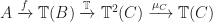
Example: For the list monad $\mathbb{L}$ , we can think of a Kleisli morphism $f : A \rightarrow B$ as producing a list of possible outputs. This can be seen as a crude form of non-deterministic computation. The identity $\mathsf{id}_A$ is the function of type $A \rightarrow \mathbb{L}(A)$ acting as:

$a \mapsto [a]$ .

So the identity “deterministically” returns its input as its output. Now if we consider two Kleisli maps $f : A \rightarrow B, g : B \rightarrow C$ , their composite acts as follows:

Input $a$ is mapped by $f$ to some list of possible outputs, say $[a_1,\ldots,a_n]$ .
The output of $f$ is transformed by applying $g$ element-wise to produce a list-of-lists $[g(a_1),\ldots,g(a_n)]$ .
The multiplication concatenates the results together into a single output list.

Encoding non-determinism via lists is favoured in many software programming contexts as they have an efficient representation as a datatype. A perhaps more satisfactory mathematical representation of (unbounded) non-determinism is the following.

Example: The Kleisli category of the powerset monad is equivalent to the category of sets and relations between them.

Example: Recall the state monad for a set $S$ , constructed from the Cartesian closure of $\mathsf{Set}$ . A Kleisli map $A \rightarrow B$ for this monad is a function of type $A \rightarrow S \Rightarrow (B \times S)$ . For $a \in A$ , $f(a)$ is a function taking a state value, and producing an element of $B$ and a new state value. The Kleisli composition of such maps does exactly what a programmer might hope, threading state and computation values through a composite of two such stateful computations.

An Algebraic Perspective

As well as this computational perspective, as has been the case for other aspects of monads, it is instructive to consider an algebraic point of view as well.

Consider an equational presentation $(\Sigma,E)$ , and the monad $\mathbb{T}$ it induces, as discussed in earlier posts. A Kleisli morphism $f : A \rightarrow B$ is a function $f : A \rightarrow \mathbb{T}(B)$ . We can think of this as an $A$ -indexed family of equivalence classes of terms with variables in $B$ , which we might write as $([t_a])_{a \in A}$ (Recall $[t]$ denotes an equivalence class with representative $t$ ). If we have a second morphism $g : B \rightarrow C$ , this is a function $g : B \rightarrow \mathbb{T}(C)$ , that is a $B$ -indexed family of terms with variables ranging over $C$ . Denote this family $([t'_b])_{b \in B}$ . The composite $g \bullet f$ will encode an $A$ -indexed family of terms with variables in $C$ . Formally, this family is:

$([t_a[t'_b / b \mid b \in B]])_{a \in A}$

Here the notation $t[t'_b / b \mid b \in B]$ denotes substituting each occurrence of variable $b$ appearing in term $t$ with $t_b$ .

So algebraically, the Kleisli category has morphisms families of (equivalence classes of) terms, and composition is substitution. From this point of view, the identity morphism at $A$ is $\eta_A$ , which corresponds to the trivial family:

$([a])_{a \in A}$

This family acts as a two sided identity with respect to substitutions as required.

The Eilenberg-Moore Adjunction

In the previous post, we introduced the Eilenberg-Moore category of a monad $\mathbb{T}$ . It is of course convenient to have mechanisms for constructing new categories, but the Eilenberg-Moore category has a more fundamental purpose. As is usual in category theory, what matters is not just individual mathematical objects, but also their relationships to others.

For a monad $\mathbb{T}$ on $\mathcal{C}$ , there is a forgetful functor from the Eilenberg-Moore category to the base category $U^{\mathbb{T}} : \mathcal{C}^{\mathbb{T}} \rightarrow \mathcal{C}$ , with action:

$U^{\mathbb{T}}(A, \alpha) = A \qquad U^{\mathbb{T}}(h) = h$

There is also a slightly less obvious free algebra functor in the other direction $F^{\mathbb{T}} : \mathcal{C} \rightarrow \mathcal{C}^{\mathbb{T}}$ , with action:

$F^{\mathbb{T}}(A) = (\mathbb{T}(A), \mu_A) \qquad F^{\mathbb{T}}(f) = \mathbb{T}(f)$

There is an adjunction $F^{\mathbb{T}} \dashv U^{\mathbb{T}}$ . To see this, we must show a natural bijection between:

Eilenberg-Moore algebra morphisms $F^{\mathbb{T}}(A) \rightarrow (B,\beta)$ .
$\mathcal{C}$ -morphism $A \rightarrow U^{\mathbb{T}}(B,\beta)$ .

In one direction, we define mapping:

$F^{\mathbb{T}}(A) \xrightarrow{h} (B,\beta) \mapsto A \xrightarrow{\eta_A} \mathbb{T}(A) \xrightarrow{h} B$

and in the the:

$A \xrightarrow{k} U(B,\beta) \mapsto F^{\mathbb{T}}(A) \xrightarrow{\mathbb{T}(k)} F^{\mathbb{T}}(B) \xrightarrow{\beta} (B,\beta)$

That this second mapping results in a valid algebra morphism follows from naturality of $\mu$ , and the Eilenberg-Moore algebra multiplication axiom. We then note that, using that $h$ is an algebra morphism, and one of the monad unit axioms:

$\beta \circ \mathbb{T}(f \circ \eta_A) = h \circ \mu_A \circ \mathbb{T}(\eta_A) = h$

In the other direction, using natural of $\eta$ , and the Eilenberg-Moore algebra unit axiom:

$\beta \circ \mathbb{T}(k) \circ \eta_A = \beta \circ \eta_B \circ k = k$

We therefore have the required bijection establishing the adjunction (leaving confirming naturality of the bijection as an exercise).

Now we consider the monad induced by this adjunction. The endofunctor action on objects is:

$U^{\mathbb{T}}F^{\mathbb{T}}(A) = U^{\mathbb{T}}(\mathbb{T}(A), \mu_A) = \mathbb{T}(A)$

On morphisms:

$U^{\mathbb{T}}F^{\mathbb{T}}(f) = U^{\mathbb{T}}(\mathbb{T}(f)) = \mathbb{T}(f)$

The unit of the monad has components the transpose of $\mathsf{id}_{F^{\mathbb{T}}(A)}$ , that is $\eta_A$ . Finally, the multiplication at $A$ is $U^{\mathbb{T}} \epsilon_{F^{\mathbb{T}}(A)}$ , with $\epsilon$ the counit of the adjunction. $\epsilon_{F^{\mathbb{T}}(A)}$ is the transpose of $\mathsf{id}_{U^{\mathbb{T}}F^{\mathbb{T}}(A)}$ , that is $\mu_A$ .

Putting all this together, we have seen that the monad induced by the Eilenberg-Moore adjunction is the original monad $\mathbb{T}$ . This establishes a point we mentioned earlier. Every adjunction induces a monad, and as we have now seen, every monad arises in this way.

Eilenberg-Moore Algebras

We shall now start to explore one of the two categories that accompany every monad. The second construction, the Kleisli category, will follow shortly after.

For a monad $\mathbb{T}$ on category $\mathcal{C}$ , an Eilenberg-Moore algebra is a $\mathcal{C}$ -object $A$ , and a $\mathcal{C}$ -morphism $\mathbb{T}(A) \rightarrow A$ , satisfying the following two axioms:

Unit axiom: $\alpha \circ \eta = \mathsf{id}$ .
Multiplication axiom: $\alpha \circ \mu = \alpha \circ \mathbb{T}(\alpha)$ .

A morphism of Eilenberg-Moore algebras $h : (A,\alpha) \rightarrow (B,\beta)$ is a $\mathcal{C}$ -morphism $h : A \rightarrow B$ such that $h \circ \alpha = \beta \circ \mathbb{T}(h)$ . Eilenberg-Moore algebras and their morphisms form a category, the Eilenberg-Moore category, denoted $\mathcal{C}^{\mathbb{T}}$ . Composition and identities are as in $\mathcal{C}$ .

To get some intuition for this definition, lets assume that the monad $\mathbb{T}$ is given by an equational presentation, with a signature consisting of a single binary operation $o$ , and no equations. For a set $A$ , $\mathbb{T}(A)$ consists of terms built up from elements of $A$ by repeated applying the operation $o$ . For example, the following are all terms:

$a, o(a_1,a_2), o(o(a_1,a_2),a_3), o(a,a)$

A function $\alpha : \mathbb{T}(A) \rightarrow A$ can be seen as a way of evaluating a term built up of elements of $A$ , to yield a new element. If we consider the unit axiom, it is equivalent to requiring:

$\alpha(a) = a$

That is, bare variables are evaluated to themselves.

To see what the multiplication axiom means, we must first introduce a bit of notation for substitution. If $t$ is a term, we shall write $t[t'/x]$ for the term resulting from substituting $t'$ for each occurrence of $x$ in $t$ . For example:

$o(x,y)[o(z,z)/x] = o(o(z,z),y)$

We shall also write $t[t_x / x \mid x \in X]$ a shorthand for multiple simultaneous substitutions, when it is well-defined to do so. For example if $t_{w} = o(y,y)$ and $t_{x} = o(z,z)$ , then:

$o(w,x)[t_i/ i \mid i \in \{ w, x \}] = o(o(y,y),o(z,z))$

The multiplication axiom is then equivalent to requiring:

$\alpha(t[t_x/ x \mid x \in X]) = \alpha(t[\alpha(t_x) / x \mid x \in X]$

So evaluating a composite term can be broken up into evaluating sub-terms and then evaluating the parent term to combine the results. For example, we must have:

$\alpha(o(o(y,y),o(z,z)) = \alpha(o(\alpha(o(y,y), \alpha(o(z,z)))$

These two axioms force $\alpha$ to behave exactly as if it had picked a binary function $o^A : A \times A \rightarrow A$ , and then evaluates all terms by recursively applying $o^A$ in the obvious way.

For our example, we only required the set of equations to be empty to avoid lots of distracting equivalence class brackets everywhere. For a general equational presentation $(\Sigma,E)$ , the axioms again force that the Eilenberg-Moore algebras must evaluate by recursively applying fixed functions for each operation symbol. The quotient by provable equality simply forces that terms that are provably equal syntactically are evaluated to the same value.

Example: For the list monad, an Eilenberg-Moore algebra on $A$ is a function $\mathbb{L}(A) \xrightarrow{\alpha} A$ such that

$\alpha([a]) = a$ .
$\alpha(\mathsf{concat}([l_1,\ldots,l_n])) = \alpha([\alpha(l_1),\ldots,\alpha(l_n)])$ .

Example: For a closure operator $c : P \rightarrow P$ , the Eilenberg-Moore algebras are elements $p \in P$ such that $c(p) \leq p$ . The two axioms are trivial in this case. As every closure operator has $p \leq c(p)$ , by irreflexivity, the Eilenberg-Moore algebras can be identified with the elements of the form $c(p)$ , the closed elements of $P$ .

The list monad is the free monoid monad.

The title of this post is a common sort of remark that is made about monads. Similar examples might be:

The multiset monad is the free commutative monoid monad.
The finite powerset monad is the free join semilattice monad.

Sorting out what statements such as these mean is our current purpose. In order to do so, we need to admit to being a little bit naughty up until now. Any good category theory book or course will quickly tell you that it is important not to just consider mathematical structures, but also the transformations between them. In the earlier posts, there was a lot of discussion of monads, but no mention of what the morphisms between them might be. Without pinning this down, we cannot compare monads in any meaningful way.

Monad Morphisms

There are actually a few choices for maps between monads. We shall consider the simplest case, morphisms between monads over some fixed base category $\mathcal{C}$ . More complex notions of transformation of monads are also useful, and tend to form 2-categories rather than mere categories. We shall return to this topic again later.

A monad morphism $\sigma : \mathbb{S} \rightarrow \mathbb{T}$ is a natural transformation between the underlying endofunctors $\sigma : \mathbb{S} \Rightarrow \mathbb{T}$ satisfying two axioms:

Unit axiom: $\sigma \circ \eta^{\mathbb{S}} = \eta^{\mathbb{T}}$ .
Multiplication axiom: $\sigma \circ \mu^{\mathbb{S}} = \mu^{\mathbb{T}} \circ \sigma_{\mathbb{T}} \circ \mathbb{T}\sigma$ .

We mentioned in an earlier post that a monad can be seen as a monoid in a precise sense. From that point of view, monad morphisms are exactly monoid morphisms. Again, we shall avoid getting into the details of these statements. For now, it is sufficient to think of a monad morphism as a natural transformation between the underlying endofunctors that interacts well with the additional monad structure.

Example: For any monad $\mathbb{T}$ , the monad unit is a monad morphism $\mathsf{Id} \rightarrow \mathbb{T}$ , from the identity monad into $\mathbb{T}$ .

Example: The identity natural transformation is a monad morphism, and monad morphisms are closed under composition as natural transformations. That is, monads on $\mathcal{C}$ and monad morphisms between them form a category.

Example: If $\sigma: \mathbb{S} \rightarrow \mathbb{T}$ is a monad morphism, and it has an inverse as a natural transformation, the inverse is also a monad morphism.

Lists and free monoids

Now we have addressed the issue of monad morphisms, we are ready to show how the list monad is the free monoid monad. Recall that the free monoid monad was given forming equivalence classes of terms induced by an equational presentation $(\Sigma,E)$ of the theory of monoids. We shall denote this monad $\mathbb{T}$ . The list monad has universe $\mathbb{L}(X)$ consisting of (some set theoretic encoding of) lists of elements from $X$ . $\mathbb{T}(X)$ and $\mathbb{L}(X)$ aren’t equal, so we must consider a more liberal notion of being “the same”. There is a natural transformation $\sigma : \mathbb{T} \Rightarrow \mathbb{L}$ given inductively by:

$\sigma([1]) = []$ .
$\sigma([x]) = [x]$ .
$\sigma([t_1 + t_2]) = \mathsf{concat}(\sigma([t_1]), \sigma([t_2]))$ .

Here, $\mathsf{concat}(xs,ys)$ denotes the concatenation of the two input lists. The notation is also a bit unfortunate as square brackets denote both equivalence classes of terms, and lists of values. Intuitively, all $\sigma$ does is form a list of all the variables appearing in any representative of the equivalence class, in the order which they appear from left to right. The axioms of the theory of monoids ensure this is a well defined map, and in fact it is a monad morphism. $\sigma$ has an inverse given inductively on lists by:

$\sigma^{-1}([]) = [1]$ .
$\sigma^{-1}(x:xs) = [x] +^{F(X)} \sigma^{-1}(xs)$ .

Here $x:xs$ is list formation via the usual cons operation you might see in Haskell for example.

So we have seen that the list monad “is” the free monoid monad in that they are isomorphic as monads on $\mathsf{Set}$ . The analogous statements about the free commutative monoid and free join semilattice monads arise via similar arguments. (Of course, there is a lot more to check than I’ve done explicitly here, that the maps are well defined, that they are natural, that the monad morphism axioms hold,…).

There are other senses in which the list monad is the free monoid monad, but to discuss those, we will need to introduce the Eilenberg-Moore category of a monad, which we shall discuss in a later post.